March 2010 - Page 3 of 5 - Math and Multimedia

GeoGebra Tutorial 9 – Vector and Translation

March 17, 2010 GB GeoGebra, High School Geometry, Software Tutorials

This is the ninth tutorial in the GeoGebra Intermediate Tutorial Series. If this is your first time to use GeoGebra, you might want to read the GeoGebra Essentials Series.

In this tutorial, we use the Vector between Two Points tool to translate a triangle and investigate the relationship between its preimage and image. We will also use the grid in this tutorial.

If you want to follow this tutorial step-by-step, you may open the GeoGebra window in your browser by clicking here.

	1.) Open GeoGebra and select the Algebra & Graphics view from the Perspectives menu.
	2.) Display the grid by clicking the View menu and choosing Grid.
	3.) Click the New Point tool and place the points on the coordinates given: A on (2,3), B on (4,1) and C on (5,2).
	4.) Next, we draw triangle ABC using the Polygon tool. To do this, click the Polygon tool and click the points in the following order: point A, point B, point C and point A again to close the polygon.
	5.) To display the label and the coordinates of the points, right click the points then click Object Properties to display the Preferences dialog box.
	6.) In the Basic tab of the Preferences dialog box, check the Show label check box, and choose the Name & Value option in the drop-down list box, and then close the window. Your drawing should look like the figure below. Figure 1
	7.) The only remaining part of the construction is the vector tool. To construct vector DE, select the Vector between Two Points tool, click the origin and click the coordinate (1,2). After this step, your drawing should look like the one shown in Figure 2. Figure 2
	8.) To translate the object using the vector, select the Translate Object by Vector tool, click the triangle and then click the vector. Notice that a translated triangle appears after clicking the vector tool.
	9.) What can you say about the preimage of the triangle object and the translated object?
	10.) If the coordinates of the vertices of the translated triangle is not displayed, display it using the steps we have done in step 5 and 6.
	11.) What do you observe about the relationship of the coordinates of the points of the original triangle and the translated triangle?
	12. Move the terminal point (point E) of the vector. Does your observation in (11) still hold?

10 comments example of vectors, GeoGebra, GeoGebra translate object tool, GeoGebra Tutorial, geometric transformation, geometric translation, vector

An extensive explanation about the Epsilon-Delta definition of limits

March 15, 2010 GB Calculus and Analysis, College Mathematics

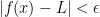One of the most important topics in elementary calculus is the $\epsilon-\delta$ definition of limits. The definition says that the $\lim_{x \to a} f(x)= L$ if and only if, for all $\epsilon > 0$ , there exists a $\delta >0$ such that if $|x-a| < \delta$ , then $|f(x) - L |<\epsilon$ . In this article, we are going to discuss what this definition means. Readers of this article must have knowledge about elementary calculus and the concept of limits.

Review of Limit Basics

Consider the function $f(x) = 2x$ . We have learned from elementary calculus that $\lim_{x \to 2} 2x = 4$ . Aside from algebraic computation, this is evident from the color-coded graph and the table shown in Figure 1. The yellow arrows in the graph and the values in the yellow cells in the table indicate that as the value of $x$ approaches $2$ from the left of the x-axis, the value of $f(x)$ approaches $4$ from below of the y-axis. On the other hand, the red arrows in the graph and the values in the red cells in the table indicate that as the value of $x$ approaches $2$ on from the right of the x-axis, the value of $f(x)$ approaches $4$ from above of the y-axis.

Figure 1 – The table and the graph showing the value of f(x) as x approaches 2 from both sides.

From the above discussion, it is noteworthy to mention three things:

We can get $f(x)$ as close to $4$ as we please by choosing an $x$ sufficiently close to $2$ . For example, I can set $x$ to $1.9999 \cdots99$ (with $100$ nines) to get an $f(x)$ very close to $4$ , which is $3.9999 \cdots 98$ ( $99$ nines).
No matter how small is the distance of $x$ from $2$ , a distance less than it may still be chosen. For example, if we choose the point which is very close to $2$ , say a point with coordinate $1.9999 \cdots 99$ with ( $100$ nines), we can still choose a value closer than this to $2$ . For instance, we can choose $1.9999 \cdots 99$ with $101$ nines. This can be repeated for every chosen distance.
Although $x$ can be very very close to $2$ , it does not necessarily mean that $x$ equals $2$ .

Now we go back to the definition of limits. In a specific example, the limit definition states that the $\lim_{x \to 2} 2x = 4$ if (and only if) for all distance (denoted by the Greek letter $\epsilon$ ) from $4$ along the y-axis (directly above or below $4$ ) – no matter how small – we can always find a certain distance (denoted by $\delta$ ) from $2$ along the x-axis (left or right of $2$ ) such that if $x$ is between $2 - \delta$ and $2 + \delta$ , then $f(x)$ would lie between $4 - \epsilon$ and $4 + \epsilon$ .

To give you a more concrete example, suppose we want the distance $\epsilon$ from $4$ , which is our limit, to be $0.1$ then the interval of our $f(x)$ is ( $4 -0.1, 4+ 0.1) = (3.9,4.1)$ . The definition of limit says that given a distance $\epsilon = 0.1$ , we can find a distance $\delta$ in the x-axis such that if $x$ is between $2 - \delta$ and $2 + \delta$ , we are sure that $f(x)$ is between $3.9$ and $4.1$ . We do not know the value of $\delta$ yet, but we will calculate it later.

Figure 2 – The epsilon-delta definition given epsilon = 0.1.

In Figure 2, $x$ is between 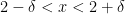$2 - \delta$ and $2 + \delta$ or $2 - \delta < x < 2 + \delta$ . Subtracting $2$ from all terms of the inequality, we have 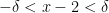$- \delta < x - 2 < \delta$ . If you recall the definition of absolute value, this is precisely the same as $|x - 2| < \delta$ . The comparison among the notations is in Table 1.

Using the notations in the table, we can conclude that the following statements are equivalent:

Words: Given $\epsilon = 0.1$ , we can find a $\delta$ such that if $x$ is between $2 - \delta, 2 + \delta$ , then $f(x)$ is between $3.9$ and $4.1$ .
Set Notation: Given $\epsilon = 0.1$ , we can find a $\delta$ such that if $x \in (2 -\delta, 2 + \delta)$ , then $f(x) \in (3.9,4.1)$ .
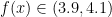Relational Operator: Given $\epsilon = 0.1$ , we can find a $\delta$ such that if $2 - \delta < x < 2 + \delta$ , then $3.9< f(x) < 4 .1$ .
Absolute Value: Given $\epsilon = 0.1$ , we can find a $\delta$ such that if $|x-2| < \delta$ , then $|f(x) - 4| < 0.1$ .

We have discussed that we can get $f(x)$ as close to $4$ as we please

by choosing an $x$ sufficiently close to $2$ . This is equivalent to choosing an extremely small $\epsilon$ , no matter how small, as long as $\epsilon>0$ . Our next task is to find the $\delta$ that corresponds to that $\epsilon$ .

Applying this definition to our example, we can say the $\lim_{x \to 2} 2x = 4$ if and only if, given $\epsilon > 0$ (any small distance above and below 4), we can find a $\delta > 0$ (any distance from x to the left and right of $2$ ) such that if $|x - 2| < \delta$ , then $|f(x) - 4| < \epsilon$ .

The Definition of a Limit of a Function

Now, notice that $4$ is the limit of the function as $x$ approaches $2$ . If we let the limit of a function be equal to $L$ and $a$ be the fixed value that $x$ approaches, then we can say that $\lim_{x \to a} f(x) = L$ if and only if, for any $\epsilon>0$ (any small distance above and below $L$ ), we can find a $\delta>0$ (any small distance from to the left and to the right of a) such that if $|x - a| < \delta$ then, $|f(x) - L| < \epsilon$ . And that is precisely, the definition of limits that we have stated in the first paragraph of this article.

Figure 3 – The epsilon-delta definition given any epsilon.

In mathematics, the phrase “for any” is the same as “for all” and is denoted by the symbol $\forall$ . In addition, the phrase “we can find” is also the same as “there exists” and is denoted by the symbol $\exists$ . So, rephrasing the definition above, we have $\lim_{x \to a} f(x) = L$ if and only if, $\forall \epsilon > 0, \exists \delta >0$ , such that if $|x - a| < \delta$ then, $|f(x) - L| < \epsilon$ . A much shorter version of this definition is the phrase $\lim_{x \to a} f(x) = L \iff, \forall \epsilon > 0, \exists \delta >0$ , such that $|x - a| < \delta \Rightarrow |f(x) - L| < \epsilon$ . The symbol $\iff$ stands for if and only if and the symbol $\Rightarrow$ is similiar to if-then. If $P$ and $Q$ are statements, the statement $P \Rightarrow Q$ is the same as the statement of the form “If $P$ then $Q$ “.

Finding a specific delta

We said that given any positive $\epsilon$ , we can find a specific $\delta$ , no matter how small our $\epsilon$ is. So let us try our first specific value $\epsilon = 0.1$ .

From the definition, we have $\lim_{x \to 2} 2x = 4$ if and only if, given $\epsilon> 0$ (any small distance above and below 4), $\exists \delta >0$ such that if $|x -2| < \delta$ then, $|f(x) - 4| < \epsilon$ .

Now $|f(x) - 4| = |2x - 4| < \epsilon$ . This implies that
$|2||x-2| < \epsilon$ which implies that $2|x - 2| <0.1$ . Simplifying, we have $|x- 2| < 0.05$ . This means that our $x$ should be between $1.95$ and $2.05$ to be sure that our $f(x)$ is between $3.9$ and $4.1$ . This is shown in Figure 4.

Figure 4 – The table showing some of the values of epsilon and delta satisfying the definition of limit of 2x as x approaches 2.

Now, let $\epsilon = 0.05$ . This means that our interval is $(3.95,4.05)$ . Now $|f(x) - 4| = |2x - 4| < 0.05$ . Thus, $|2||x -2| < \epsilon$ which implies that $2|x - 2| <0.05$ . Solving, we have $|x - 2| < 0.025$ . This means that our $x$ should be between $1.975$ and $2.025$ to be sure that our $f(x)$ is between $3.95$ and $4.05$ . There are only two examples above, but the definition tells us that we can choose any $\epsilon > 0$ so let us generalize our statement by doing so.

Now $|f(x) - 4| = |2x - 4| < \epsilon$ . This results to $|2||x -2| < \epsilon$ which implies that $2|x - 2| <\epsilon$ . Solving, we have $|x - 2| < \epsilon/2$ . From the condition above, $|x - 2| < \delta$ so we can let $\delta = \epsilon/2$ .

This means given any $\epsilon$ , we just let our $\delta$ equal to $\epsilon/2$ and we are sure that if $x$ is between $2-\delta/2$ and $2+\delta$ to be sure that our $f(x)$ is between $4 - \epsilon$ and $4 - \epsilon$ .

In the next calculus post, we are going to discuss the strategies on how to get $\delta$ given an arbitrary $\epsilon$ value, so keep posted.

Related Articles

23 comments absolute value, concept of limits, definition of limits, epsilon-delta definition, epsilon-delta explanation, epsilon-delta proof, relational operators, representation of limits, set notation

GeoGebra Basic Construction 2 – Isosceles Triangle

March 12, 2010 GB GeoGebra, Software Tutorials

There are many ways to construct an isosceles triangle using GeoGebra. The concept in this construction is mathematical, so making a similar construction in other dynamic geometry software is more or less the same. Some geometry software will probably differ a little bit which will depend on how the tools are used in construction.

In this tutorial, we learn one way: To create a circle and use the center of the circle and two points on its circumference to form an isosceles triangle.

Figure 1 – Isosceles Triangle ABC.

The idea is to create a circle with radius AB, create point C on the circle and connect the vertices with the Polygon tool. The last step is to hide the circle. If you have used GeoGebra before, then this will be very easy.

	1.) Open GeoGebra and select Geometry from the Perspectives menu in the Sidebar.
	2.) Click the Circle with Center through Point tool and click two distinct places on the Graphics view to construct a circle with center A and passing through point B.
	3.) If the labels of the points are not displayed, click the Move tool, right click each point and click Show label from the context menu. Notice that GeoGebra automatically names the points in alphabetical order.
	4.) Select the Point tool and click the circumference of the circle to construct point C. Figure 2 – Circle with center A and passing throught points B and C.
	5.) Drag the three points and observe the difference among the three. What do you observe?
	6.) To draw the triangle, click the Polygon tool, click point A, click point B, click point C and click point A again to close the polygon.
	7.) Next, we hide the circle by right clicking its circumference and unchecking Show Object from the context menu.
	8.) Drag the vertices of the triangle. What do you observe? Why is triangle *ABC* and isosceles triangle?

Point C is an example of dependent objects in GeoGebra. Unlike points A and B, point C can only move along the circumference of the circle. Hence, AC will depend on the length of radius AB. In addition, since point C is dependent on the circumference of the circle, once you delete the circle, point C will also be deleted. This is not the same the other way around. Even if you delete point C, the circle will still remain.

Points A and B, on the other hand, are independent objects. Independent objects are not “attached” to other objects. You can drag them anywhere without restrictions.

If you have used GeoGebra before, it is possible to construct an isosceles triangle in other ways. Some of the tools that you can use are:

Angle Bisector tool
Perpendicular Bisector tool
Midpoint tool
Compass Tool

4 comments dynamic geometry sofware, GeoGebra, geogebra geometry, GeoGebra Tutorial Series, isosceles triangle

« 1 2 3 4 5 »