Introduction
One of the most fundamental problems that gave birth to integral calculus was the calculation of areas bounded by curves. The Greeks used method of exhaustion to remedy this problem, particularly on finding the area of a circle. After Descartes’ and Fermat’s invention of Coordinate Geometry, algebraic solutions were utilized.

One of the strategies used to find the area under the function  between
  and
and  is to divide it into sub-intervals and form rectangles as shown in the first figure. Clearly, as the number of rectangles increases, the sum of all the areas of the rectangles gets closer and closer to the area of under the curve.
A Specific Case
To explain further, let us take a specific case of the function  and find the area under the curve bounded by
  ,
,  , and the x-axis. As we have mentioned above, we will divide the intervals, and for convenience, we use equal intervals, and construct rectangles as shown in the second figure. In this case, we see to it that the upper left corner of all the rectangles touch the graph; the right graph or the center of the graph may also be used.

If we let  and
and  be the areas of the rectangles above (ordered from left to right), then the total area of the rectangles are

which equals

using the summation notation.
If we let  and
and  be the coordinates of the leftmost part of the rectangles, then the upper left corner of the first rectangle that touches the graph have coordinates
  where
where  is its height (Can you see why?). The base of the rectangle is
  . If we let
  , the base of the rectangle, then the area of the first rectangle is
  . Using this notation, the sum of the areas of the five rectangles is

which is equal to
 .
.
Now, we note two things. First, the sum of the areas of all the rectangles between the  and always less than the area under the curve. Second, as we have mentioned above, as we increase the number of rectangles, the better our approximation.
So, to approximate the area under the curve, we create as many rectangles as we can. If we create  rectangles where for a very large , the sum of the areas of all rectangles is
 .
.
Now, as gets larger and larger, or as approaches infinity, the sum of the areas of rectangles approaches the area under the curve. In fact, the limit of the sum of the areas of the rectangles as approaches infinity is equal to the area under the curve. In calculus, the area under the curve  between
  and $x = b$ is denoted by

Using both notations, we have
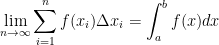 .
.
So, in our specific case above,
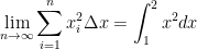 .
.
The notation means the area under the curve from to .