Free Geometry and Topology Ebooks
Below are free Geometry and Topology ebooks. Most of these books are in PDF format. Some of the links point to a website containing the ebooks, while some directly links to the pdf files. All of these ebooks are downloadable and free.
- A Text-Book of Geometry by G. A. Wentworth
- CK-12 Geometry by V. Cifarelli, A. Gloag, D. Greenberg, J. Sconyers, B.
- Geometry for Elementary School by Wikibooks
- The Elements by Euclid
College Geometry and Beyond
- A First Course in Topology: Continuity and Dimension by John McCleary
- A Tour of Triangle Geometry by Paul Yiu
- Algebraic and Geometric Topology by Andrew Ranicki, Norman Levitt, Frank Quinn
- Algebraic Curves: an Introduction to Algebraic Geometry by William Fulton
- Algebraic geometry and projective differential geometry by Joseph M. Landsberg
- Algebraic Geometry by J.S. Milne
- An Introduction to Differentiable Manifolds and Riemannian Geometry by William M. Boothby
- An Introduction to Riemannian Geometry by Sigmundur Gudmundsson
- Classical Geometry by Danny Calegari
- Computational Geometry
- Course of Differential Geometry by Ruslan Sharipov
- Elementary Topology O. Ya. Viro, O. A. Ivanov, N. Yu. Netsvetaev, V. M. Kharlamov
- Fractal Geometry by Michael Frame, Benoit Mandelbrot, Nial Neger
- Fundamentals of Geometry by Oleg A. Belyaev
- Geometric Asymptotics
- Geometry and Billiards by Serge Tabachnikov
- Geometry and Group Theory
- Geometry and Quantum Field Theory by Pavel Etingof
- Geometry Formulas and Facts by Silvio Levy
- Geometry study guide
- Geometry of Surfaces Nigel Hitchin
- Geometry of the Sphere by John C. Polking
- Geometry, Topology, Geometric Modeling by Jean Gallier
- Geometry Unbound Kiran S. Kedlaya
- Intrinsic Geometry of Surfaces by A. D. Aleksandrov and V. A. Zalgaller
- Introduction to Symplectic and Hamiltonian Geometry by Ana Cannas da Silva
- Natural Operations in Differential Geometry Ivan Kolar, Peter W. Michor, Jan Slovak
- Non-Euclidean Geometry by Henry Manning
- Open Problems in Topology by Jan Van Mill, George M. Reed
- Projective and Polar Spaces by Peter J. Cameron
- Projective Differential Geometry Old and New by V. Ovsienko, S. Tabachnikov
- Projective Geometry by Nigel Hitchin
- Riemann surfaces, dynamics and geometry Course Notes
- The Eightfold Way: The Beauty of Klein’s Quartic Curve editedy by Silvio Levy
- The Foundations of Geometry by David Hilbert
- The Geometry and Topology of Three-Manifolds William P Thurston
- The Geometry of Iterated Loop Spaces by J. P. May
- Topics in Finite Geometry: Ovals, Ovoids and Generalized Quadrangles by S. E. Payne
- Topology and Geometry for Physics by H. Eschrig
- Topology Without Tears by Sydney A. Morris
You may also want to view my list of Free Algebra and Free Calculus ebooks.

 be the width of our rectangle, it follows that the length is
  . Let
. Let  be the area of the rectangle. In effect, the area of the rectangle is described by the equation
  . We want to maximize the area, which implies that we want to find the maximum value of
 , which we will denote
  . We then equate the
  resulting to the equation
  which is exactly the maximum value in the table above.
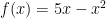 . To give a clearer picture let us look at the graph of

 = 100 km – 50 km over the difference in time
 = 10:00 – 8:00. This is shown in the figure below. This is equivalent to 50 km/2 hrs or 25 km/hr. From the computation above, it is clear that the interpretation of the slope of the secant line is the total distance over the total time or the average speed.