Compound Interest and the Irrational Number e
Suppose we borrow Php* 1.00 from a loan company at an interest rate of 100% a year, then after a year we would have to pay Php 2.00. We have learned from elementary school mathematics that to get the interest, we have to multiply the principal by the rate. Just in case, we already have forgotten, the computation to calculate the interest is shown below.

Figure 1 – Computation of the Interest of 1.00 given a rate of 100% a year.
*Php stands for Philippine pesos, the currency in my country.
The situation above is an example of a simple interest problem. Simple interest is calculated by multiplying a fixed interest rate to a principal amount over a fixed period of time.
There are several scenarios that could happen in loaning money. Most of the loan companies accept early payments; some allow the borrowers to re-borrow the money, and some apply interests to amount payable just like re-borrowing money. Let us see what happens in both scenarios.
Scenario 1: Paying Early
Suppose you borrowed money for 1 year and luckily you got money after 6 months, and you want to pay your loan immediately. Your loan company might only charge you 50% such as shown in Figure 2.

Figure 2 – Computation of Interest of 1.00 peso compounded semiannually at a rate of 100% a year.
Scenario 2: Re-borrowing Money
Another scenario is to borrow the money for six months and re-borrow it again for another six months without paying the first loan. Note that this is the same as failing to pay a six-month loan for a year. The question is, after borrowing 1 peso for six months with an interest of 50% the first six months and another 50% in the second six months, do you think your loan company will let you pay Php 2.00 for 1 year? Well – lucky you are if they do.

Table 1 – Computation of 1 peso loan compounded semi-annually at an annual rate of 100% interest.
Loan interests do not work that way. That is because from scenario 1, after 6 months, the amount that you have to pay the company is Php 1.50. Hence, if you re-borrow the money without paying the principal – or you failed to pay it for another six months – the principal amount during your second loan will not be Php 1.00 but Php 1.50. The computation of this scenario is shown in the table in Table 1 and is called compound interest. That is applying the interest rate not only to the principal amount (which Php 1.00 in the first six months), but also including the interest (which is Php 0.50 in the first six months).
If we have a fixed rate, say 100% (or 1 in decimal equivalent), then we have to divide it into the number of times that we are going to compound our interest in one year. For instance, applying a 100% interest to a one-year loan compounded monthly will require us to divide 100% by 12 which is 8.5% per month or 0.085 in decimal equivalent. Table 2 shows the computation of this scenario. In January, the principal is only Php 1.00 and after applying the interest, the amount payable is 1.085. That means, if you want to pay at the end your January, you have to pay 1.085 or 1.09 pesos. This becomes the principal amount in February. If we multiply 1.085 by 0.085, our interest in February is 0.092. If we add this to the principal amount in February, which is 1.085, then the amount payable by the end of February is 1.177 peso or 1.18 pesos.

Table 2 – Computation of Interests of a 1-peso loan compounded monthly at a 100% annual interest rate.
This process is repeated until December. As shown in the table, by the end of December, 2.66 is the amount payable for the 1-peso loan for 1 year with 100% interest compounded monthly.
Generalization
Putting the principal and interest in table in Figure 3 into computation, we have the following.

Figure 3 – Computation of Amount Payables given the number of compounds per year.
Looking at Figure 3, in the January row of Table 2, we have a principal of 1 and an interest rate of 0.085 = 1/12. Thus, using the pattern shown in Figure 3, in general, if we have 1 as principal, 100% as annual interest, and n as the number of times we are going to compound the interest in a year, then the amount payable after a year can be computed by the formula 
- What happens as the number of compound is getting larger and larger? What happens if we compound per day, per hour, per minute and per second?
- What happens if we divide 1 (that is, 100%) into a very large number? Will the amount payable reach a very large number? Will amount payable reach infinity?
Using 1-peso as principal and 1 (or 100%) as interest per year, the table below shows the amount payable given the number of times the interest is compounded in a year. As we can see, compounding daily gives approximately 2.714 pesos and compounding every second 2.718, only a difference of 0.004. It is evident that as the number of compounds of year increases, the smaller the increase in amount payable per year.
Does that mean that the amount payable is approaching a particular number?

Table 3 – Computation of Amount Payables given the number of compounds per year.
Also, from the table, it seems that as the number of compounds increases, the amount payable is approaching 2.7182818. In fact, raising the number of compounds per year to 1 billion gives us 2.7182820, an increase of 0.02. This means, that this number has a limit as we increase the number of compounds per year.
The number that is the limit of the expression 
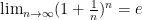

 and
and  , it is clear that the length of CD is
  units. To determine the midpoint of CD, we want to get the coordinates of the point which is
  units away from both points C and D. Hence, we have to divide
  or subtract the result from
  . Summarizing, the expression that would describe the value of the y-coordinate of the midpoint would be
  or
or  . This means that the midpoint of CD is
  .
. or
or  . This means that the midpoint of AB is
  .
.
 and
and  (see Figure 2), we can get its midpoint using the following formula
  or
or 

 . Similarly, for a horizontal segment with endpoints having coordinates
  and
and  can be computed by the expression
  .
. .
. which is the midpoint of RS. From here, it is tempting to ask the following question:
 ?
?
 and B
and B  equal to
  ?”
?”

 and the coordinates of B are
  , the coordinates of M is equal to
 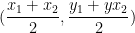 .
. and
and  lies on the midpoint formula. The details of the solutions are left to the reader as an exercise.
 all the way up to
  , it is quite cumbersome to write
  . Mathematical notations permit us to shorten such addition using the
  symbol to denote “all the way up to” or “all the way down to”. Using the this symbol, the expression above can be written as
  .
. as shown below.

 is the last index and
  is the variable. We use the letter
  as our index variable, or the variable that will hold the changing quantities. Hence, if we are going to use the sigma or the summation notation for the expression

 is the same as
  and is the same as
  .
. and so on.


 equals
  which means that
 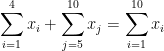 . In general,
  .
.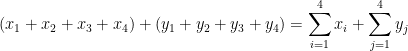 . Regrouping the expression, we have
 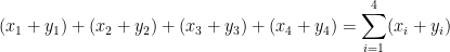 . This means that
  Generalizing, we have
 (
( of them)
  . But
. But  (
( . Therefore,
  .
. . But
. But 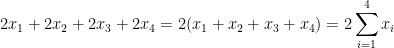 . In general,
 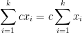 .
.