GeoGebra Tutorial 14 – Sliders and Circle-Area Approximation

This is the 14th tutorial in the GeoGebra Tutorial Series. If this is your first time to use GeoGebra, I suggest that you read the GeoGebra Essentials series first.

In this tutorial, we use GeoGebra to approximate the area of a circle.  This strategy of approximating the area of a circle was used by the Greek mathematician Archimedes.

Since this tutorial is long, we split it into two parts. In Part I, we inscribe a regular polygon in a circle, increase its number of sides, and investigate the relationship between the areas. In Part II we will circumscribe the circle with a regular polygon increase its number of sides to approximate the circle’s area.  Before following the tutorial step-by-step, click here to view the final output.

Part I – Creating an Inscribed Polygon

Step-by-Step Instructions

1. Open GeoGebra click on Algebra & Graphics in the Perspectives menu
2. In this tutorial, we want all new objects to be labeled. To do this, click the Options menu, click Labeling, then click on All New Objects.
3. Next, we create  slider r that will determine the radius of the circle that we are about to create.  Select the Slider tool, then click anywhere on the Graphics view to display the Slider dialog box.
4. In the Slider dialog box, type r in the Name box, type 0.1 in the min box, and leave the max value as 5 and increment as 0.1, then click the Apply button.

5. Create another slider name it n, set the minimum to 3, maximum to 30 and increment to 1. Slider n will determine the number of sides of the inscribed polygon.
6. Next, we create point A on the origin. To do this, select the Intersect Two Objects Tool, click the x-axis and then click the y-axis.
7. To construct a circle with center A and radius r, type circle[A,r] . Move slider r and observe what happens.
8. To construct point which is the intersection of the circle and the x-axis, type B = (r,0) in the input box and press the ENTER/RETURN key on the keyboard.
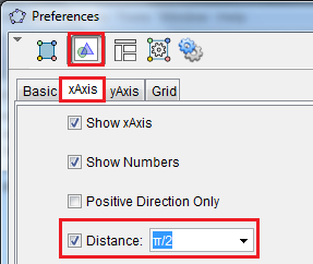
9. Now, we compute for the central angle of the inscribed polygon. To do this, we divide 360 by n. For example, if we want to have an equilateral triangle, we must divide 360 by 3, which will be the central angle. To do this, type a = (360/n)° then press the ENTER key. The degree sign, tells GeoGebra that a is an angle measure. You can display the ° sign can be written by clicking the \alpha button at the right of the input box.
10.  To create angle BAB’, click the Angle with Given Size tool, click on point B and then click on point A. This will display the Angle with Given Size dialog box.
11.  In the Angle dialog box, type a in the Angle text box,  choose the counterclockwise option, and then click the OK button. If you set r to 3, your drawing should look like the one shown in Figure 2.

Figure 2 – Central angle BAB’.

12.  To hide the angle measure (green sector), right click it then click Show Object.
13.  To construct the inscribed polygon, select the Regular Polygon tool, click B and then click B’. This will display the Regular Polygon dialog box.
14.  In the Regular Polygon dialog box, type n and then click the OK button. Now, drag slider n and see what happens. If you setto 30 and to 3, the figure should look like Figure 3.

Figure 3 – A circle with an inscribed 30-sided polygon.

15.  The problem now is to hide the labels of all the points and the segments. With n set to 30, right click the polygon, then click Object Properties from the context menu to display the Preferences dialog box.
16.  In the Preferences dialog box, select the Basic tab, click Point (be sure that the Point text is highlighted) in the Objects list, and uncheck the Show Label check box. This will hide the labels of all the points. Now, click Segment text in the Objects check box and uncheck the Show Label check box to hide the labels of all the sides of the polygons, then click the Close button.

GeoGebra Preferences Dialog Box

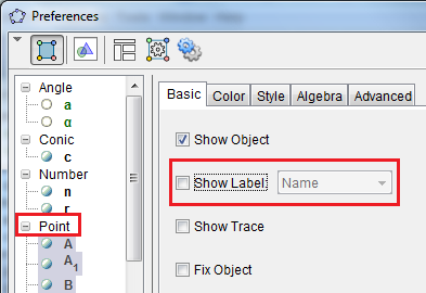
Figure 4 – The GeoGebra Preferences dialog box.

Exercise:

  1. Move the slider and observe what happens.
  2. Using the text tool, display the area of the circle and the area of the inscribed triangle.Your drawing should look like Figure 5.

Figure 5 – Final Output

GeoGebra Tutorial 12 – Pictures and Angle Measures

This is the 12th tutorial in the GeoGebra Intermediate Tutorial Series. If this is your first time to use GeoGebra, you may want to read the GeoGebra Essentials Series.

In this tutorial, we learn how to use the Insert Image tool. We insert  an image of a protractor in the Graphics view, create two connected segments,  and measure the angles formed by two segments. We use the Check Box the Text tools to show or hide the actual measure to see if the approximation of the applet’s user is correct. The final output of this tutorial is ideal for elementary school students for practicing their estimation skills on measuring angles.

In this tutorial, we learn the following:

  1. Use new tools: The Insert Image and the Semicircle through Two Points tool.
  2. Show/hide objects using a check box.
  3. Combine the text and variable using the text tool to display measures of angles.

You can view the final output of the tutorial here.

Step-by-Step Instructions

1. Open GeoGebra and click on Algebra & Graphics in the Perspectives menu.
2. We set GeoGebra to label new points only and not other objects. To do this, click the Options menu, click Labeling, then click New Points Only.
3. Click the New Point tool, click the origin and click on (12,0). Notice that GeoGebra automatically names the points in alphabetical order. The point on the  A and the other B.
4. Click the Line through Two Points tool, click point A and then click point B. Now, hide the coordinate Axes by clicking the Axes button at the upper left of the Graphics view (click the arrow if not displayed).
5. To create a semicircle passing through points A and B, click the Semicircle through Two Points tool click point A and click point B. Your drawing should look like Figure 1.

Figure 1 – Semicircle passing through points A and B.

6. To get the midpoint C of AB, select the Midpoint or Center tool, click point A and click point B.

7. Now, create two more points on the semicircle. To do this, select the New Point tool and click two different locations on the circumference of the semicircle to produce points D and E.
8. Now, create radii CD and CE by click the Segment between Two Points tool, click point C and click point D to connect CD. With the segment tool still active, click point C and point E to construct segment CE.
9. To display the measure of angle DCE, select the Angle tool, click segment CE, then click segment CD. GeoGebra will automatically name DCE angle \alpha.

Figure 2 – Angle measure of DCE.

10.  Next, hide the measure of angle DCE. To do this, click the Show/Hide Label tool, then click the angle measure (the green sector).
11.  Next, we hide points A and B and the semicircle. To do this, select the Show/Hide Object, click point A, point B, and the semicircle. Notice that all the clicked object are highlighted. Click the Move button to hide them.
12.  Now, let us insert the image. Select the Insert Image tool, click anywhere on the Graphics view. In the Open dialog box, search and click the protractor image, click it and then click the Open button. This will display the protractor.  Your GeoGebra window look like the one shown in Figure 3.

Figure 3 – The Protractor image in the drawing pad.

13.  We now create a text that will display the measure of angle DCE. To do this, click the Insert Text tool, click anywhere on the drawing pad to display the text tool dialog box.
14.  In the Text dialog box, type the following:

The measure of angle DCE is \alpha is \alpha

The first \alpha symbol can be inserted by selecting it in the Symbol drop down box (see figure)  below the Edit box. This will display the Greek letter \alpha. The second \alpha is the measure of the angle. It can be inserted using the Objects drop-down box.

GeoGebra Text Tool

The second α will display the angle measure of DCE.

15.  Next, we construct a check box that will display or hide the text that we have constructed. To do this, click the Checkbox to Show/Hide Objects tool and click anywhere on the Graphics view to display the check box dialog box.
16.  In the dialog box, type Show/Hide measure of angle DCE and choose Text Text1 from the Select objects… drop down list box, then click the Apply button.Figure 4

17.  Now, be sure that the check box is unchecked to hide the angle measure of angle DCE.  Move points D and E. Use the Move button to adjust the protractor to measure angle DCE. Guess the measure of angle DCE.

Figure 5 – Protractor measuring angle DCE.

18.  Click the check box to see if your approximation is correct.

The protractor image used in this applet was from MathisFun.com. Before doing   his tutorial, you need a picture of a protractor preferably in png format and with white background.


GeoGebra Tutorial 11 – Sliders and Graphs of Trigonometric Functions

This is the eleventh tutorial in the GeoGebra Intermediate Tutorial Series. If this is your first time to use GeoGebra, you may want to read the GeoGebra Essentials Series.

In this tutorial (now updated to GeoGebra 4.2), we use sliders to explore the effects of the parameters a, b, c and d of the graph f(x) = a sin(bxc) + d, g(x) = a cos(bxc) + d and h(x) = a tan(bxc) + d. We also learn about a new tool, the Checkbox to Show/Hide Objects tool. The output of this tutorial is shown in Figure 1.  If you want to explore first before following the tutorial, the GeoGebra applet can be viewed here.

Figure 1 – The graphs of the sine, cosine and tangent functions with similar values of a, b, c and d.

Although this tutorial is the eleventh of the GeoGebra Tutorial Series, it is a stand-alone tutorial. You may follow it step-by-step without having to learn the previous ten.

Instructions

1.) Open GeoGebra and click on the Algebra & Graphics at the Perspectives menu.
2.) First, we create assigned values to a, b, c and d. These numbers will be our slider later. To assign a number to a, type a = 1 in the Input bar, then press the ENTER key. Now, construct numbers b, c, and d by typing b = 1, c = 1, and d = 1 and press the ENTER key after each equation.
3.) To create sliders a, b, c and d, right click each one of them in the Algebra view and click Show object from the context menu.

GeoGebra Sliders

4.) Before graphing the functions, change the interval of the x-axis from 1 to π/2. To do this, right-click any blank space on the Graphics view and click on Graphics… from the context menu to display the Settings dialog box.

5.) In the Settings dialog box, select the Graphics section,  click the x-axis tab, check the Distance check box, select π/2 from the Distance drop-down list box, and then close the dialog box.

preferences

6.) Now, to graph the sine function, type f(x) = a*sin(b*x-c)+d in the Input bar, then press the ENTER key. In GeoGebra, the * symbol stands for multiplication.
7.) To graph the cosine and tangent function, type g(x) = a*cos(b*x-c)+d,then press the ENTER key and type h(x) = a*tan(b*x-c)+d then press the ENTER key.
8.) Move sliders a, b, c and d. What do you observe? How does a, b, c and d affect the graph of the sine function, the cosine function and the tangent function?
9.) Next, we create three check boxes that will show or hide the graphs of the three trigonometric functions. To create a check box that will show/hide the sine function, select the Check Box to Show/Hide Object tool, then click anywhere on the Graphics view to display the Check Box to Show/Hide Objects dialog box.
10.)  In the Check box dialog box, type Show/Hide Sine Function in the Caption box,  click the sine graph in the Graphics view, and then click the  Apply button to finish. Notice that the sine function appears on the list box.

Figure 5 – The Check Box to Show/Hide Objects dialog box.

11. )   Select the Move tool and click the check box several times. What do you observe?
12. )   Using steps 9-10, create two more check boxes for the cosine function and the tangent function.
13.)    Next, we show the grid. We can use the grid to approximate the x and y values of a particular point. To do this, click the View menu, then click Grid.
14.)   Lastly,  change the color of the graphs to distinguish them easily.
1 36 37 38 39 40 44