solving quadratic equations Archives

Derivation of the Quadratic Formula

December 18, 2009 GB High School Algebra, Questions and Quandaries

When we discuss about functions, we usually talk about their roots, or geometrically where their graphs pass through the x-axis. For example, $- 3, 1$ and $3$ are the roots of the graph of the function in Figure 1 because it passes through $x = -3, x =1$ and $x=3$ .

Since we are looking for points on the x-axis, it means that all the points that we are looking for have $y$ -coordinate $0$ . As a consequence, (i) if we want to find the root of a quadratic function we have set $y = 0$ and then solve for the values of $x$ .

Figure 1 – The x-axis and the line with equation y = 0 are basically the same line so all points on the x-axis have y-coordinate 0.

With the things above in mind, let us find the roots of two quadratic functions: $(1) y = x^2 + 5x + 6$ and $(2) y = x^2 + 3x + 1$ .

Finding the root by Factoring

The roots of the function $y = x^2 + 5x + 6$ are easy to find. As we have said, to get the root of a function, we set $y$ to $0$ and then find the value the value of $x$ . Solving by factoring, we have

$x^2 + 5x + 6 = 0 \Rightarrow (x + 2)(x + 3) = 0$

Now, $(x + 2)(x + 3) = 0$ if $x + 2 = 0$ or/and $x + 3 = 0$ . Solving for the value of $x$ on both equations, we have $x= -2$ and $x = -3$ .

Thus, even though we have not seen the graph of the function yet $y = x^2 + 5x + 6$ , we are sure that it will pass through $x = -2$ and $x = -3$ . If you want to verify if the graph of the function $y= x^2 + 5x + 6$ indeed passes through the $x$ -axis at $x = -2$ and $x = -3$ , you can verify its graph using a graphing software or a graphing calculator.

Figure 2 – We are sure that the graph of $y = x^2 + 5x + 6$ will pass through the yellow points.

Factoring: Another Interpretation

Another possible interpretation of the expression $x^2 + 5x + 6$ can be the area of a rectangle with length $x + 3$ and width $x+2$ . The distribution of the products of the terms of the expressions are represented by the four rectangles formed shown below.

Figure 3 – Another interpretation of the expression x^2 + 5x + 6.

Let us try another example: Let us find the roots of the quadratic function $y = x^2 + 3x + 1$ . You will probably observe that there is no way that we can factor this expression. The last term is $1$ , but there are only two factors of 1: $\{1,1\}$ and $\{-1,-1\}$ , so this means that that the numerical coefficient of $x$ must be $2$ or $-2$ , but it is equal to $3$ . Hence, the expression is not factorable.

Since, the expression is not factorable, we cannot find the length and width of a rectangle with area $x^2 + 3x + 1$ . The easiest way probably to find its length and width is to assume that it is a square.

Completing the Square

We have a quadratic expression which we assumed a perfect square so its factor must be of the form $(x+b)(x+b)$ where $b$ is a real number. Also, $(x+b)^2 = x^2 + 2bx + b^2$ . If we consider $x + b$ as a side of the square, then the product of the expressions will form two squares namely $x^2$ and $b^2$ , and 2 congruent rectangles with each having an area of $bx$ .

Figure 4 – A square with side x + b, where b is a constant.

If we want to use the product of $x+ b$ above, first, we have to take off $x^2$ as one of the squares. Then we are left with a figure with area $3x$ which we will divide into two congruent rectangles. If we are going to follow the positions of the rectangles in Figure 4, then we will have an $x^2$ and two pieces of $\frac{3}{2}x$ (see Figure 5).To construct a square, we extend one of the sides of each of the congruent rectangles.

Figure 5: Completing the square of x^2 + 3x + 1.

Since we have two small rectangles with area $\frac{3}{2}x$ , and the longer side (in the diagram) is $x$ , it follows that the other dimension is $\frac{3}{2}$ which gives us a smaller square with area $\frac{9}{4}$ .

Figure 6 – The area of the small formed is 9/4 and the side length of the big square formed is x + 3/2.

The biggest square formed in Figure 6 has area $x^2 + \frac{3}{2}x +\frac{9}{4}$ , which is $\frac{5}{4}$ more than our original quadratic expression, so we will deduct $\frac{5}{4}$ to preserve the original expression. So our final expression is $x^2 + \frac{3}{2}x +\frac{9}{4} - \frac{5}{4}$

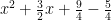
Algebraically, if we have the expression $x^2 + bx + c$ , and we want to “compete its square”, we want to transform it to an expression of the form $(x-h)^2 + k$ . For example, $x^2 + 6x + 12$ can be expressed as $(x + 3)^2 + 3$ . Another example is that $x^2 + 8x + 12$ can be written as $(x + 4)^2 - 4$ . Note that the coefficient of $x^2$ should be $1$ so that we are sure that a square $x$ by $x$ is formed as shown in figures 4,5 and 6. In general, the possible steps that we are going to create using the general equation $y = ax^2 + bx + c$ is to set $y$ to $0$ and then find the value of $x$ .

In constructing the square in Figure 6, we went through the following processes:

(ii) We made sure that the numerical coefficient of $x^2$ is $1$ to ensure that we have a square with factors (side length) $x$ .

(iii) We isolated the constant term $c = 1$ , and we just used the first $x^2$ and the second term $3x$ .

(iv) To get the area of the smaller square, we divided the numerical coefficient of the $3x$ by $2$ then squared it to get $\frac{9}{4}$ .

Shown in Figure 7 is the summary of the steps we did to get the roots of the quadratic function $y = x^2 + 3x + 1$ . The rightmost column of the table shows the generalization of our steps, which is getting the roots of the quadratic function $y = ax^2 + bx + c$ .

Figure 7 – A step-by-step derivation of the quadratic formula.

Quadratic Formula

The formula 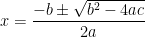$x = \displaystyle\frac{-b \pm \sqrt{b^2-4ac}}{2a}$ located at the bottom part of the rightmost column of the table in Figure 7 is called the quadratic formula. We have derived the quadratic formula from completing the square of a quadratic equation. From the formula, the roots o the quadratic function $y = ax^2 + bx + c$ are $\displaystyle\frac{-b + \sqrt{b^2-4ac}}{2a}$ and $\displaystyle\frac{-b - \sqrt{b^2-4ac}}{2a}$ .

10 comments completing the square, completing the square method, derivation of quaratic formula, factoring, factoring trinomials, perfect square trinomial, quadratic completing the square, quadratic equations roots, quadratic formula, quadratic function, quadratic polynomial roots, roots of a quadratic function, solving quadratic equations, solving quadratic formula