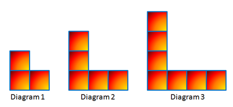
Problem: Consider the diagrams below. If the pattern continues, how many squares will there be in Diagram 50? Diagram 100?

Figure 1 - A sequence of L-shaped square blocks.
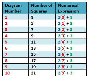
In solving problems, it is important to present data in which we can easily see patterns. Table 1 shows the relationship between the diagram numbers and the number of squares.

Table 1 – The relationship between the diagram number and the number of squares.
We can solve this problem by “brute force” extending the table up to Figure 100, but that is not very “mathematical.” What mathematics had taught us is to find patterns, and, if possible, make generalizations. Using the first term, the constant difference and the diagram number, we can form a numerical expression that when simplified will result to the number of squares as shown in Table 2. Looking at the table, we can see that the first term is 3, and the difference is 2. Using this pattern, it is now easy to compute the number of squares of any diagram number.
Examine the table and see if you can find the pattern before proceeding.

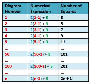
Table 2 - Numerical expressions describing the number of squares in each diagram number.
In Table 2, we can see that in the numerical expression column, the constant difference 2 and the first term 3 appear in every term. The changing quantity (variable) is the figure number – 1. Using the pattern, it is easy to see that the 50th term is 2(50-1) + 3= 101 and the 100th term is 2(100-1) + 3 = 201. In general, Figure n will have 2(n-1) + 3 = 2n + 1 squares.

Table 3 – Generalized expression describing the number of squares.
Let us denote the nth term of a sequence by tn. Since 2 and 3 are constants, if we let a be the first term of the sequence and d be the constant difference, then the formula that will describe the nth term of the sequence is
tn = a(n-1) + d
Arithmetic Sequence as a Linear Function
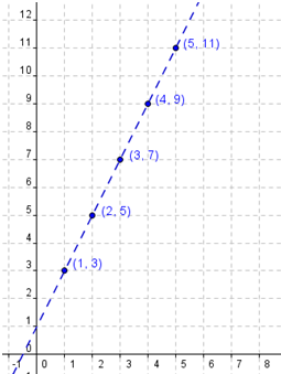
Figure 2 shows the graph of the arithmetic sequence and its trend line denoted by the dashed line. Since we have a constant difference, we have a linear function. If we want to get the equation of the linear function that describes the relationship in our problem, since several ordered pairs are given, we can use the slope intercept formula.

Figure 2 – Graph of the d(n) = 2n + 1, where d(n) is the diagram number
If we extend the trend line, it will pass the (0,1) (Why?). Getting (1,3) as our second point, the slope m will be (3-1)/(1-0) = 2. Hence, the equation of our line will be y = 2x + 1 which is of the same form as tn = 2n + 1 in Table 3.

