Slope Concept 2 – Slope of the Graph of a Linear Function

Note: This is the second part  of the the Slope Concept Series. The second and third articles are Part I – Understanding the Basic Concepts of Slope and Part III – Slopes of Vertical and Horizontal Lines.

***

In the Understanding the Basic Concepts of Slope post, we have discussed that slope is described as rise over run. In this post, we are going to show that the slope of a straight line is constant.

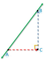
To get the slope of a straight line or a segment, we determine two points on the line, say A and B, draw a horizontal line through point A and a vertical segment through point B. We then determine the intersection of the two line segments and name it C as shown in Figure 1. Angle C is a right angle since BC is a vertical segment and AC is a horizontal segment.

Figure 1 - A line containing points A and B.

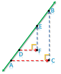
The slope of the line containing AB is \frac{BC}{AC}. If we determine two more points, say D and E on the line, and do the process mentioned above, we can come up with triangle DEF right angled at F as shown in Figure 2. In terms of DEF, the slope of the line containing points D and E is \frac{EF}{DF}. Since the line containing DE and AB is practically the same line, we have learned from high school mathematics that their slopes must be equal.  Hence, the following relationship holds: \frac{BC}{AC} = \frac{EF}{DF}.

Why is this so?

Figure 2 - Triangle ABC and DEF with their hypotenuse contained on the line.

To show that the slope of the line is constant, we must show that \frac{BC}{AC} =\frac{EF}{DF}.

Proof That the Slope of a Straight Line is Constant

From Figure 2, BC is parallel to EF, since they are both vertical segments.  Similarly, DF is parallel to AC, since they are both horizontal segments. By the Parallel Postulate, we can consider AB as a transversal of the two pairs of parallel segments.

We can see that angles DEF and ABC are congruent since they are corresponding angles. Angles C and F are also congruent since they are both right angles. Hence, by AA similarity, ABC is similar to DEF.  Since the ratio of the corresponding sides of a similar triangles are equal, it follows that \frac{BC}{AC} =\frac{EF}{DF}.

From the above proof, we have shown that the slope of a straight line, or the slope of the graph of a linear function,  is constant.

Introduction to the Concept of Functions

Problem: A cube is painted on all faces and cut into smaller cubes of the same size. Investigate the number of painted faces of the smaller cubes.

Discussion

In Figure 1, shown are the cubes with side lengths two units and three units. The light blue cube has been painted and cut into eight smaller unit cubes, while the yellow cube has been painted yellow and cut into 27 smaller unit cubes. To avoid confusion, we will simply call the bigger or uncut cubes “cube”and the smaller cubes “unit cubes”.

How many unit cubes can be formed from a painted cube with length 4 units? 5 units? n units?
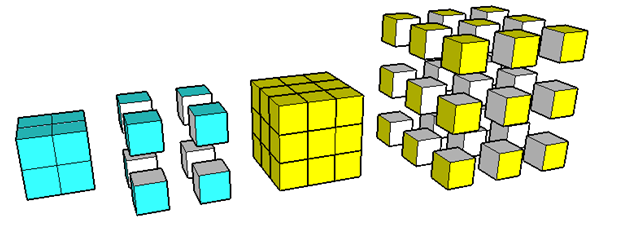
Figure 1 – Cubes with side lengths 2 and 3 cut into unit cubes.

Before scrolling down, investigate the number of painted faces of each yellow unit cube. In Figure 2, the unit cubes have been drawn from different perspectives to make visualization easier.

How many cubes are there with 3 painted faces? 2 painted faces? 1 painted face? 0 painted face?
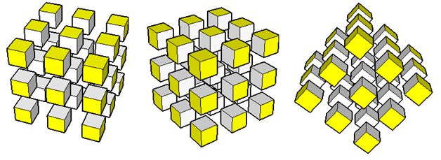
Figure 2 – Cube cut into 27 unit cubes shown in different perspectives.

Without drawing, can you determine the number of painted faces of a cube with side length 4 units? How about 5 units? 6 units?

Challenge: Find a formula for the number of unit cubes 3 painted faces, 2 painted faces, 1 painted face and 0 painted face given a side length n units.

To determine how many unit cubes are painted given a particular size, it will help us if we know the properties of a cube. Let us recall that a cube has 8 vertices, 6 faces and 12 edges.
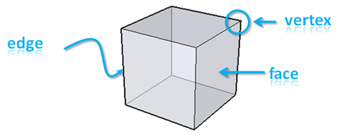
Figure 3 – Parts of a cube.

For the sake of discussion, we will name and color the unit cubes (see Figure 4) and group them depending on their positions – whether they are at the edges, vertices or faces of the cube.

  • Vertex Cubes (Red) – are the unit cubes located at the vertices of the cube. It is evident only 3 of their faces are painted.
  • Edge Cubes (Green) – are the unit cubes located at the 12 edges of the cube. Note that only two of their faces are painted.
  • Wall Cubes (Blue) – are the unit cubes at the faces of the cube. We will call the wall cubes because we will use the word “face” in another context.
  • Core Cubes (No color) – are cubes that are at the core of the cube that was not painted.

Figure 4 – The cube showing number of painted faces depending on their positions.

From Figure 4, it is clear that vertex cubes have 3 painted faces, edge cubes have 2 painted faces, wall cubes have 1 painted face and core cubes have no painted face.

Extending this type of grouping to cubes of larger side lengths, a pattern can be seen as shown in the table below. The calculation for the number of cubes can be generalized.

Figure 5 – Table showing the relationship of the number of painted faces given the cube’s sidel length.

Let us make the following definitions:

a = number of core cubes of an cube with side length n

b = number of wall cubes of a cube with side length n

c = number of edge cubes of a cube with side length n

d = the number vertex cubes with side length n

then

a = (n – 2)3 = n3 – 9n2 + 27n – 27

b = 6(n-2)2 = 6n2 – 24n + 24

c = 12(n-1) = 12n- 12

d = 8

That means that we have created a formula for finding the number of painted faces no matter how large it is. For example, if we want to find the number of wall cubes in from a cut cube with length 100 units, then there are a = 6(100)2 – 24(100) + 24 = 57624 wall cubes.

Question: If m is the volume of the cube before it was cut, then how can you express m in terms of a,  b, c and d?

Let us consider first the equation c = 12(n-1) = 12n – 12. Note that for each side length n, there is a corresponding number of edge cubes denoted by c. And there is only one c. For instance, if n = 3, there is no other value for c except 24. And clearly, this is true for all values of n.

If for each n there is exactly one corresponding c, then we say that c is a function of n.  Hence, we describe what a function means:

A function is a relationship between two sets where for every element of the first set, there is exactly one corresponding element in the second set.

In our case, our first set is the side length of the cube which is n, and our second set is the number of edge cubes that we denoted by c.   In general, if we have set A and set B, for every element in A, there is exactly one corresponding element in B.

The symbol f(x) is read as “f of x” and is usually used as a notation of a function.

We now denote the functions a as f(x), b as g(x), c as h(x) and d as k(x).

We will now graph our functions in the xy plane. The graphs of these functions are shown in Figure 6. The dots represent the ordered pairs and the dashed lines and curves are the lines that we will be formed if we will let x be the set of real numbers instead of integers.

Figure 6 – The points and the trendlines of the graphs of f(x), g(x), h(x) and k(x).

Summary

In this article, we have learned the following:

  • A function is a relationship between varying quantities.
  • A function is a relationship between two sets where for each element in the first set, there is exactly one corresponding element in the second set.
  • A function maybe represented as a table, set of ordered pairs such as (3,8), (4,8), (5,8), equations and graphs.

In the sequel of this article, we will discuss more about the basics of functions and its properties, so keep posted.

Geometer’s Sketchpad Tutorial 3: Graphs and Sliders

In this tutorial, we are going to use Geometer’s Sketchpad to explore the graph of the function y = mx + b where m and b are real numbers. First, we are going to type each equation manually, but later, we are going to use sliders to see the relationship between the parameters m and b and the appearance of the graph.

Steps Graphing Equations

  1. Open Geometer’s Sketchpad.
  2. Click the Graph menu from the menu bar and click Define Coordinate System from the  list.
  3. To graph the function y = 2x, click the Graph menu, then click Plot New Function to display the New Function dialog box.
  4. In the New Function dialog box, type 2x, then click the OK button.

Figure 1 – The New Function dialog box.

Using steps 1 through 4, graph the following functions and observe how the value of m affects the graph of y = mx

  1. y = 3x
  2. y = 4x
  3. y = 5x
  4. y = 10 x
  5. y = – 2x
  6. y = – 4x
  7. y = -6x
  8. y = – 10x

Graph the following functions and observe how b affects the graph of the function y = mx + b.

  1. y = 2x + 3
  2. y = 2x + 1
  3. y = 2x + 5
  4. y = 2x – 1
  5. y = 2x – 4
  6. f. y = 2x – 10

Creating a Slider

There is a better way to explore the relationship of the parameters of functions and their graphs. Instead of typing each equation, we can use the sliders to assign values to parameters like m and b. A slider is a visual representation of a number. For instance, if you have a slider m with domain -10 through 10, then moving the slider rightward will increase the value of m. The slider that we will create here is very similar to Graphs and Sliders 1 and Graphs and Sliders 2 posts in the GeoGebra Tutorial Series.

The construction of slider in Geometer’s Sketchpad is somewhat different compared to the slider in GeoGebra. We will use the idea of ratio in creating a slider here.  To create a slider, we will construct segment AB, and construct point C on AB. We will divide the measure of AC by the measure of AB,then multiply it to 20. This means that our minimum value is 0 and our  maximum number is 20. To facilitate negative values, we will subtract 10 from result of our computation. This means that our minimum value is 0 – 10 = -10 and our maximum value is 20 – 10 = 10.

If you want to extend the domain of your slider, you just multiply the quotient of AC and AB by your desired number and subtract half of that desired number from the product.

Figure 2 – The slider control consisting of point C on segment AB.

Steps in Constructing a Slider

  1. Open Geometer’s Sketchpad.
  2. To show the coordinate axes, click the Graph menu from the menu bar and click Define Coordinate System from the drop-down list.
  3. To construct our slider, click the Segment tool from the toolbox, and construct a horizontal segment on the drawing area.
  4. To display the label of the two points, select the two points, click the Display menu from the menu bar and click Show Labels from the list.
  5. To construct point C on AB, click the Point tool and click segment AB (not the points).
  6. Display the label of point C, by right clicking it and choosing Show label from the pop-up menu.
  7. For our computation of the value of m, we first measure the value of AC and AB. To measure AC, select points A and C (be sure that only the two points are selected), click the Measure menu and click Distance from the list.
  8. To measure AB, select points A and B, then click the Measure menu and click Distance from the list.
  9. Figure 3 – The Measure-Distance command displays the distance between two points.

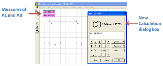
  10. To find the value of m, we divide AC by AB, multiply the result to 20 and the subtract 10. To do this, click the Measure menu and click Calculate from the list.
  11. Click the text on the drawing area displaying the measure of AC, click the ÷ button from the New Calculation dialog box, click the label displaying the measure of AB, click * from the New Calculation dialog box, then type 20-10, then click the OK button on the dialog box when finished.  This will be our value of m.
  12. Figure 4 – The New Calculation dialog box.

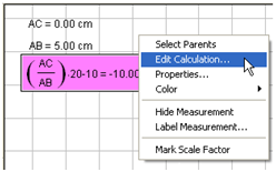
  13. Move point C and observe what happens to the value of m. If you want to Edit your calculation, just click the Arrow tool, right click the the value of m, then click Edit Calculation.
  14. Figure 5 – The pop-up menu that appears when you right click the value of m.

  15. To graph y = mx, click the Graph menu, then click Plot New Function to display the Plot New Function dialog box.
  16. While the Plot New Function box is displayed, click the label containing the value of m, click the * button, click the x (or type x), then click the OK button. If you have followed the steps correcty, the graph of y = mx should appear in your coordinate system.
  17. Hide points A and B and the labels containing the values of AB and AC by clicking the Display menu and click Hide Objects.
  18. Move point C. What do you observe? What relationship can you conclude between the value of m and the appearance of the graph of the function?

Exercise:

  1. Construct another slider for the value of b.
  2. Construct a graph that will display the value of f(x) = mx + b.
  3. Describe the effect of b in the graph of the function f(x) = mx + b.
1 2 3 4