In this tutorial, we are going to use Geometer’s Sketchpad to explore the graph of the function y = mx + b where m and b are real numbers. First, we are going to type each equation manually, but later, we are going to use sliders to see the relationship between the parameters m and b and the appearance of the graph.
Steps Graphing Equations
- Open Geometer’s Sketchpad.
- Click the Graph menu from the menu bar and click Define Coordinate System from the list.
- To graph the function y = 2x, click the Graph menu, then click Plot New Function to display the New Function dialog box.
- In the New Function dialog box, type 2x, then click the OK button.

Figure 1 – The New Function dialog box.
Using steps 1 through 4, graph the following functions and observe how the value of m affects the graph of y = mx
- y = 3x
- y = 4x
- y = 5x
- y = 10 x
- y = – 2x
- y = – 4x
- y = -6x
- y = – 10x
Graph the following functions and observe how b affects the graph of the function y = mx + b.
- y = 2x + 3
- y = 2x + 1
- y = 2x + 5
- y = 2x – 1
- y = 2x – 4
- f. y = 2x – 10
Creating a Slider
There is a better way to explore the relationship of the parameters of functions and their graphs. Instead of typing each equation, we can use the sliders to assign values to parameters like m and b. A slider is a visual representation of a number. For instance, if you have a slider m with domain -10 through 10, then moving the slider rightward will increase the value of m. The slider that we will create here is very similar to Graphs and Sliders 1 and Graphs and Sliders 2 posts in the GeoGebra Tutorial Series.
The construction of slider in Geometer’s Sketchpad is somewhat different compared to the slider in GeoGebra. We will use the idea of ratio in creating a slider here. To create a slider, we will construct segment AB, and construct point C on AB. We will divide the measure of AC by the measure of AB,then multiply it to 20. This means that our minimum value is 0 and our maximum number is 20. To facilitate negative values, we will subtract 10 from result of our computation. This means that our minimum value is 0 – 10 = -10 and our maximum value is 20 – 10 = 10.
If you want to extend the domain of your slider, you just multiply the quotient of AC and AB by your desired number and subtract half of that desired number from the product.

Figure 2 – The slider control consisting of point C on segment AB.
Steps in Constructing a Slider
- Open Geometer’s Sketchpad.
- To show the coordinate axes, click the Graph menu from the menu bar and click Define Coordinate System from the drop-down list.
- To construct our slider, click the Segment tool from the toolbox, and construct a horizontal segment on the drawing area.
- To display the label of the two points, select the two points, click the Display menu from the menu bar and click Show Labels from the list.
- To construct point C on AB, click the Point tool and click segment AB (not the points).
- Display the label of point C, by right clicking it and choosing Show label from the pop-up menu.
- For our computation of the value of m, we first measure the value of AC and AB. To measure AC, select points A and C (be sure that only the two points are selected), click the Measure menu and click Distance from the list.
- To measure AB, select points A and B, then click the Measure menu and click Distance from the list.

Figure 3 – The Measure-Distance command displays the distance between two points.
- To find the value of m, we divide AC by AB, multiply the result to 20 and the subtract 10. To do this, click the Measure menu and click Calculate from the list.
- Click the text on the drawing area displaying the measure of AC, click the ÷ button from the New Calculation dialog box, click the label displaying the measure of AB, click * from the New Calculation dialog box, then type 20-10, then click the OK button on the dialog box when finished. This will be our value of m.

Figure 4 – The New Calculation dialog box.
- Move point C and observe what happens to the value of m. If you want to Edit your calculation, just click the Arrow tool, right click the the value of m, then click Edit Calculation.

Figure 5 – The pop-up menu that appears when you right click the value of m.
- To graph y = mx, click the Graph menu, then click Plot New Function to display the Plot New Function dialog box.
- While the Plot New Function box is displayed, click the label containing the value of m, click the * button, click the x (or type x), then click the OK button. If you have followed the steps correcty, the graph of y = mx should appear in your coordinate system.
- Hide points A and B and the labels containing the values of AB and AC by clicking the Display menu and click Hide Objects.
- Move point C. What do you observe? What relationship can you conclude between the value of m and the appearance of the graph of the function?
Exercise:
- Construct another slider for the value of b.
- Construct a graph that will display the value of f(x) = mx + b.
- Describe the effect of b in the graph of the function f(x) = mx + b.

on websites, blogs and wikis. If you do not know about Latex, I have created a Latex tutorial here and here.
 equals
  is a definition. There are actually a few reasons why this is so – the two of which are shown below.
 taken
taken  letters from A, B, C and D
  . But,
 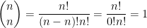 . To satisfy the equation,
  . Dividing both sides by
  . If we let
  , we have
  which is what we want to show.
 which means that


 .
.