Limit by epsilon-delta proof: Example 1

February 27, 2011 GB Calculus and Analysis, College Mathematics

We have discussed extensively the meaning of the $\epsilon-\delta$ definition. In this post, we are going to learn some strategies to prove limits of functions by definition. The meat of the proof is finding a suitable $\delta$ for all possible $\epsilon$ values.

Recall that the definition states that the limit of $f(x) = L$ as $x$ approaches $a$ , if for all $\epsilon > 0$ , however small, there exists a $\delta > 0$ such that if $0 < | x - a| < \delta$ , then $|f(x) - L| < \epsilon$ .

Example 1: Let $f(x) = 3x + 5$ . Prove that $\lim_{x \to 2} f(x) = 11$

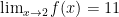
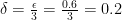
If we are going to study definition limit above, and apply it to the given function, we have $\lim_{x \to 2} 3x + 5 = 11$ , if for all $\epsilon > 0$ , however small, there exists a $\delta > 0$ such that if $0 < |x - 2| < \delta$ , then $|3x + 5 - 11| < \epsilon$ . We want to find the value of $\delta$ , in terms of $\epsilon$ ; therefore, we can manipulate one of the inequalities to the other’s form. In particular, we will manipulate $|3x + 5 - 11| < \epsilon$ to an expression such that the expression inside the absolute value sign will become $x - 2$ .

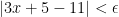
Simplifying, we have $|3x - 6| = 3|x-2|< \epsilon$ . This expression is equivalent to $3|x-2|< \epsilon$ . Dividing both sides by $3$ , we have $|x-2|< \frac{\epsilon}{3}$ . Now, both inequalities have the same form.

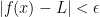
That means that whatever value of $\epsilon$ is, we can find a $\delta = \frac{\epsilon}{3}$ satisfying the conditions above. To explain further, let us have a specific example.

Let us choose a small $\epsilon = 0.6$ . From the definition, for $\epsilon = 0.6$ , there exists a $\delta=\frac{\epsilon}{3} =\frac{0.6}{3}= 0.2$ such that if $0 < | x - 2| < 0.2$ , then $|3x + 5 - 11| < 0.6$ . The geometric interpretation of this statement is shown below.

Click the picture to view GeoGebra applet by Sylvain Bérubé

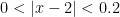
Now, let us intepret the definition. While reading these statements, look at the third diagram above:

Our $L=11$ , we have chosen $\epsilon = 0.6$ , and our computation gives us $\delta = \frac{\epsilon}{3} = \frac{0.6}{3} =0.2$ .
The statement, let $\epsilon = 0.6$ means that we are creating an interval which is $(L - \epsilon, L + \epsilon) =(11-0.6,11+0.6)= (10.4,11.6)$ . This can be seen in the y-axis.
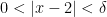
The statement $0 < |x - 2| < 0.2$ means that we are creating an interval $(a - \delta, a + \delta)=(2 -0.2,2+0.2)= (1.8, 2.2)$ . This can be seen in the x-axis
In layman’s term, for $\epsilon = 0.6$ , there exists a $\delta=0.2$ such that if we take the value a particular $x$ between $1.8$ and $2.2$ , we are sure that the corresponding $f(x)$ is between $10.4$ and $11.6$ . Recall, however, that $0.6$ is a particular value. The definition states that we can make it as small as we want and still find a suitable $\delta$ , however small, our $\epsilon$ is.
In fact a game can be developed where player A gives a particular $\epsilon$ , and player B searches for a suitable $\delta$ satisfying the definition. No matter small a value player A assigns to $\epsilon$ , we are sure that player B can always find a suitable $\delta$ satisfying the definition.

The general strategy in proving limits by $\epsilon-\delta$ definition is to manipulate the inequality $|f(x) - L| < \epsilon$ such that the expression $|f(x)-L|$ is simplified to $|x - a|$ .

To explain the $\epsilon-\delta$ definition of limits further, I will give you three or four more examples in the near future.

15 comments epsilon-delta definition, epsilon-delta explanation, epsilon-delta problems, epsilon-delta proof, epsilon-delta proof example

Limit by epsilon-delta proof: Example 1

Leave a ReplyCancel reply