Experimental and Theoretical Probability Part 2
This the second part of the series of posts on Experimental and Theoretical Probability.
In the first part of this series, we used a spreadsheet to simulate the rolling of dice 1000 times and automatically recorded the sums. We have observed that the sum frequencies are not evenly distributed (see Figure 1).
In rolling the two dice 1000 times, for example, we rolled a seven 156 times, while we only rolled a two 29 times. Well, we want to think that this is just a coincidence, so maybe we could try it one more time.
How about rolling it 2000 times?
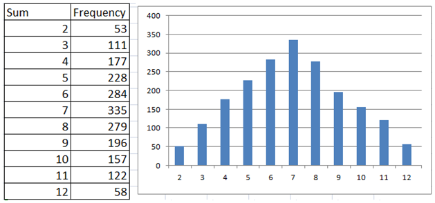
To simulate the roll 2000 times, using the steps in the previous article, we extend the random numbers to cells A2001, B2001, and C2001. Doing this in my computer(since the numbers are random, you’ll find a slightly different result), I got the sum frequency table shown in Figure 2. Still 6, 7, and 8 are the most frequent roll, while 2 and 12 remained the least. Another notable observation is that the two graphs seem to have a somewhat similar appearance.
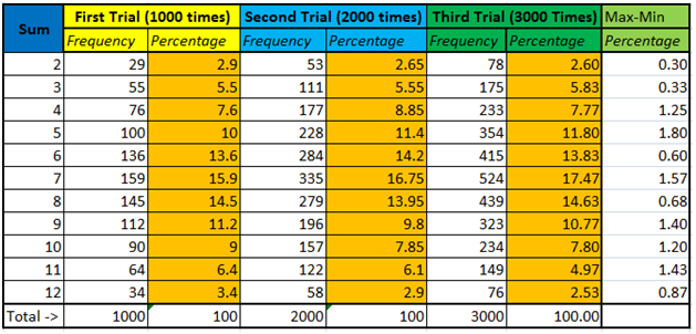
To convince myself further, I rolled the two dice 3000 times, and the result is shown in the sixth and seventh column of the table in Figure 3. Notice that in the three experiments, the percentages of rolling a particular sum, despite being random, are almost similar. Rolling a 2, for instance, ranges from 2.6 to 2.9 percent in the three experiments, and rolling a 7 ranges from 15.9 to 17.47 percent. In fact, if we subtract the minimum percentage value from the maximum percentage value of the frequencies (see last column) of all the possible sums in the three experiments, the maximum difference is only 1.8 percent. That means that the results are surprisingly consistent. Hmmm….
With the three experiments having almost similar results, there must some reasons why our results are such. That is what we are going to discuss in the third part of this series.


