GeoGebra Tutorial 11 – Sliders and Graphs of Trigonometric Functions
This is the eleventh tutorial in the GeoGebra Intermediate Tutorial Series. If this is your first time to use GeoGebra, you may want to read the GeoGebra Essentials Series.
In this tutorial (now updated to GeoGebra 4.2), we use sliders to explore the effects of the parameters a, b, c and d of the graph f(x) = a sin(bx – c) + d, g(x) = a cos(bx – c) + d and h(x) = a tan(bx – c) + d. We also learn about a new tool, the Checkbox to Show/Hide Objects tool. The output of this tutorial is shown in Figure 1. If you want to explore first before following the tutorial, the GeoGebra applet can be viewed here.

Figure 1 – The graphs of the sine, cosine and tangent functions with similar values of a, b, c and d.
Although this tutorial is the eleventh of the GeoGebra Tutorial Series, it is a stand-alone tutorial. You may follow it step-by-step without having to learn the previous ten.
Instructions
| 1.) Open GeoGebra and click on the Algebra & Graphics at the Perspectives menu. | |
| 2.) First, we create assigned values to a, b, c and d. These numbers will be our slider later. To assign a number to a, type a = 1 in the Input bar, then press the ENTER key. Now, construct numbers b, c, and d by typing b = 1, c = 1, and d = 1 and press the ENTER key after each equation. | |
| 3.) To create sliders a, b, c and d, right click each one of them in the Algebra view and click Show object from the context menu.
|
|
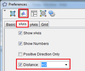
| 4.) Before graphing the functions, change the interval of the x-axis from 1 to π/2. To do this, right-click any blank space on the Graphics view and click on Graphics… from the context menu to display the Settings dialog box. | |
|
5.) In the Settings dialog box, select the Graphics section, click the x-axis tab, check the Distance check box, select π/2 from the Distance drop-down list box, and then close the dialog box.
|
|
| 6.) Now, to graph the sine function, type f(x) = a*sin(b*x-c)+d in the Input bar, then press the ENTER key. In GeoGebra, the * symbol stands for multiplication. | |
| 7.) To graph the cosine and tangent function, type g(x) = a*cos(b*x-c)+d,then press the ENTER key and type h(x) = a*tan(b*x-c)+d then press the ENTER key. | |
| 8.) Move sliders a, b, c and d. What do you observe? How does a, b, c and d affect the graph of the sine function, the cosine function and the tangent function? | |
| 9.) Next, we create three check boxes that will show or hide the graphs of the three trigonometric functions. To create a check box that will show/hide the sine function, select the Check Box to Show/Hide Object tool, then click anywhere on the Graphics view to display the Check Box to Show/Hide Objects dialog box. | |
10.) In the Check box dialog box, type Show/Hide Sine Function in the Caption box, click the sine graph in the Graphics view, and then click the Apply button to finish. Notice that the sine function appears on the list box.
 Figure 5 – The Check Box to Show/Hide Objects dialog box. |
|
| 11. ) Select the Move tool and click the check box several times. What do you observe? | |
| 12. ) Using steps 9-10, create two more check boxes for the cosine function and the tangent function. | |
| 13.) Next, we show the grid. We can use the grid to approximate the x and y values of a particular point. To do this, click the View menu, then click Grid. | |
| 14.) Lastly, change the color of the graphs to distinguish them easily. |


 . If we determine two more points, say D and E on the line, and do the process mentioned above, we can come up with triangle DEF right angled at F as shown in Figure 2. In terms of DEF, the slope of the line containing points D and E is
  . Since the line containing DE and AB is practically the same line, we have learned from high school mathematics that their slopes must be equal. Hence, the following relationship holds:
  .
.
 .
.