Slope Concept 1 – Understanding the Basic Concepts of Slope

Note: This is the first part of the the Slope Concept Series. The sequels of this article are Part II – Slope of the Graph of a Linear Function and Part III – Slopes of Vertical and Horizontal Lines.

***

The slope is known to be the steepness of a line.  Sometimes it is described as “rise over run,” If we are on point A, we go up 4 units and we go right 5 units (see Figure 1) then our rise is 4 and our run is 5. Let us mark our new location B. Notice that the order of movements does not matter. We can also go 5 units right and 4 units up and you will still be in B (see Figure 2).

If we do our movement in the coordinate plane starting from the origin, our rise would be our vertical movement (change of movement with respect to the y-axis) and our run would be our horizontal movement (change of movement with respect to the x-axis). In Figure 2, segment AB has rise 4 and run 5.  Thus, the slope of segment AB is \displaystyle\frac{4}{5}.  In general, slope in the coordinate plane is described as the change in y over the change in x.

Figure 1 - Segment AB with rise 4 units and run 5 units.

The slope of a line (or a segment) may also be described as the angle it makes with a horizontal line.  Technically speaking, it is a counterclockwise rotation with the line starting from a horizontal position about a point which is located on that line, or the origin our case.  In Figure 2, \theta is the angle measure AB makes with the horizontal axis of the rectangular coordinate plane, or the amount of rotation from AB’ to AB about A.

Figure 2 - Counter-clockwise rotation of AB to AB' about A.

Looking at triangle ABC, since the given sides are the side adjacent and the side opposite to \theta, we can use the definition of tangent to compute for the value of \theta. Recall from trigonometry that the definition of a tangent of an angle of a right triangle is equal to the quotient of the length of the side opposite to it (change in y) and the length of the side adjacent to it (change in x). Now, this is precisely the definition of slope. From here, we can conclude that the angle that a line makes with a horizontal line is the same as the slope of that line. As a consequence \tan(\theta) = \displaystyle\frac{4}{5} in radian measure (or approximately 38 degrees) is the slope of the line.

Figure 3 - Triangle ABC with Slope 4/5.

If we examine the value of \theta, it is clear that when \tan(\theta) is 0 degrees, the line is horizontal since there is no (zero) change in y. Algebraically, this makes the numerator of the fraction change in y 0 which implies that the slope of any horizontal line is 0.

If the line is vertical, there is no (zero) change in x. That makes the denominator of the fraction change in x 0. Of course, we know that anything divided by 0 is not defined. As a consequence, slope of a vertical line is undefined.

In the continuation of this article, we will discuss further about the properties of slope. We will discuss why the slope of a straight line is constant. We will further discuss zero, undefined, negative and positive slopes. We will also discuss how the concept of slope helps in solving calculus problems and how it is used to determine the behavior functions.

Area Tutorial 5 – Area of a Trapezoid

In this tutorial, we are going to derive the area of a trapezoid. A trapezoid (sometimes called a trapezium) is a quadrilateral with exactly one pair of parallel sides. Trapezoid PQRS is shown below, with PQ parallel to RS.  We have learned that the area A of the trapezoid with bases b_1 and b_2 and altitude h is given by the formula
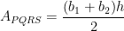
 A_{PQRS} = \displaystyle\frac{(b_1 + b_2)h}{2}.

Figure 1 - Trapezoid PQRS with PQ parallel to RS.

We are going to derive the area of a trapezoid in two ways: First by dividing into different sections and second by rotation.

Derivation 1: Area by Dividing into Regions

If we drop another line from Q, then we will have two altitudes namely PT and QU, which both have length h units.

Figure 2 - Trapezoid PQRS divided into two triangles and a rectangle.

From Figure 2, it is clear that Area of PQRS = Area of PST + Area of PQUT + Area of QRU. We have learned that the area of a triangle is the product of its base and altitude divided by 2, and the area of a rectangle is the product of its length and width. Hence, we can easily compute the area of PQRS. It is clear that A_{PQRS} = (ah/2) + b_1h + (ch/2).  Simplifying, we have  A = \displaystyle\frac{ah + 2b_1 + ch}{2}
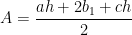
. Factoring we have, A_{PQRS} = (a + 2b_1 + c) \frac{h}{2} = [(a + b_1 + c) + b_1] \frac{h}{2}. But, a + b_1 + c is equal to b_2, the longer base of our trapezoid. Hence, A_{PQRS}= (b_1 + b_2) \frac{h}{2}.

Derivation 2: By Rotation

In the second derivation, we are going to duplicate the trapezoid and rotate it as shown below. It is evident that quadrilateral PS’P’S is a parallelogram (Why?). But we have learned that the area of the parallelogram is the product of its height and its base. Hence, A_{PS'P'S} = (b_1 + b_2)h.

Figure 3 - PQRS translated and rotated to form a parallelogram.

But the area of the trapezoid PQRS is half of the area of the parallelogram PS’P’S. Thus, A_{PQRS} = \displaystyle\frac{(b_1 + b_2)h}{2}.

Enjoy and Learn More

GeoGebra Tutorial 10 – Vectors and Tessellation

This is the 10th tutorial in the GeoGebra Intermediate Tutorial Series. If this is your first time to use GeoGebra, you might want to read first the GeoGebra Essentials Series.

This tutorial is the sequel of GeoGebra Tutorial 9 – Vector and Translation.  In this tutorial, we  use the idea of translation to tessellate  the plane. Tessellation is a process of covering a plane with no gaps and no overlaps.

The final output of our tutorial is shown in Figure 1 and the GeoGebra applet can be viewed here.

geogebra vector translation1

Figure 1 – Octagon and squares tessellating the plane.

To give you the whole picture, I have enumerated the summary of what we are going to do in this construction.

  1. Construct an octagon containing points A at (0,5) and B at (0,4).
  2. Draw point O at the origin which is the initial point of vector, P at the positive x-axis and vector Q at the negative y-axis. P and Q are the terminal points of the vectors.
  3. Draw vectors u (containing O and P) and v (containing O and Q).
  4. Translate the octagon to tessellate the plane using vector u.
  5. Translate all the created octagons down using vector v.
  6. Draw a square that will cover the space at the center of the 4 leftmost adjacent octagons.
  7. Translate the square to the right using vector u.

Construction Protocol

1.) Open GeoGebra and select Algebra & Graphics from the Perspectives menu
2.) Click the New Point tool and place two points in the coordinates given: A on (0,5) and B in (0,4).
3.) Select the Regular Polygon tool, click point A, then click point B to display the Regular Polygon dialog box. In the dialog box, type 8, then press the OK button. If the labels of the points and the segments are displayed, remove them by right clicking them and unchecking on Show label from the context menu.

Figure 2 – Octagon with containing segment AB.

4.) Next, we create three points which will be the initial and terminal points of the vector (see Figure 1). Click the New Point tool, click on the origin, click a point on the positive x-axis near the origin and the negative y-axis near the origin.
5.) We now rename the three points. To rename the point on the origin, right click it and click Rename from the context menu. In the Rename box, type O and press the OK button. Rename the point on the x-axis as P and the point on the y-axis Q.
6.) Now, to create vector u, select the Vector between Two Points tool, click on point O, then click on point P. To create vector v, with the Vector between Two Points tool still active, click point O and then click point Q to create vector v.
7.) To translate the octagon to the right, select the Translate Object by Vector tool, click the interior of the octagon, then click vector u.

8.) Adjust vector u such that the right vertical side of the first octagon coincides with the left vertical side of the translated octagon. Your drawing should look like Figure 3.

vector translation

Figure 3 – An octagon and its translation using vector u.

9.) To translate another octagon, with the Translate Object by Vector tool still active, click the rightmost octagon, then click vector u. Repeat this step three times giving us 5 octagons with adjacent vertical sides.
10.)  Next, we translate the octagons down vertically. To do this, select the Translate Object by Vector tool, click the leftmost octagon and then click vector v. Adjust the translated octagon by moving point Q such that the lower horizontal side of the original octagon coincides with the upper horizontal side of the translated octagon.
11.)  Repeat step 10 until all the 5 octagons are translated down.  After step 11, your figure should look like Figure 1 with white squares.
12.)  The last part of the task is to cover the empty square spaces between octagons. To do this, click the Regular Polygon tool, click the two consecutive points of the leftmost square (on the side of the octagon) to display the Regular Polygon dialog box.
13.)  Type 4 as the number of Vertices and then click OK. If the square created is on the other side, undo the step, and reverse the order of the click.
14. ) To tessellate, click the square and then click vector u. Repeat the translation as you have done in step 9.


1 2 3 4 5