An Intuitive Introduction to Limits
Limits is one of the most fundamental concepts of calculus. The foundation of calculus was not entirely solid during the time of Leibniz and Newton, but later developments on the concept, particularly the 
Circumference and Limits
If we are going to approximate the circumference of a circle using the perimeter of an inscribed polygon, even without computation, we can observe that as the number of sides of the polygon increases, the better the approximation. In fact, we can make the perimeter of the polygon as close as we please to the circumference of the circle by choosing a sufficiently large number of sides. Notice that no matter how large the number of sides our polygon has, its perimeter will never exceed or equal the circumference of the circle.

Figure 1 – As the number of side of the polygons increases, its perimeter gets closer to the circumference of the circle.
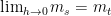
In a more technical term, we say that the limit of the perimeter of the inscribed polygon as the number of its sides increases without bound (or as the number of sides of the inscribed polygon approaches infinity) is equal to the circumference of the circle. In symbol, if we let 


Functions and Limits
Consider the function 


Figure 2 – As x increases, f(x) gets closer and closer to 0.
First, we see that as the value of 

Hence, we say that the limit of 


Tangent line and Limits
Recall that the slope of a line is its “rise” over its “run”. The formula of slope 


Figure 3 – Line n is tangent to the function f at point P.
If we are going to compute for the slope of the line tangent line, we have a big problem because we only have one point, and the slope formula requires two points. To deal with this problem, we select a point 


Figure 4 – As point Q approaches P, the slope of the secant line is getting closer and closer to the slope of the tangent line.
If we let 


Area and Limits
Another ancient problem is about finding the area under a curve as shown in the leftmost graph in Figure 5. During the ancient time, finding the area of a curved plane was impossible.

Figure 5 – As the number of rectangles increases, the sum of the area of the rectangles is getting closer and closer to the area of the bounded plane under the curve.
We can approximate the area above in the first graph in Figure 5 by constructing rectangles under the curve such that one of the corners of the rectangle touches the graph as shown in the second and third graph in Figure 5. We can see that as we increase the number of rectangles, the better is our approximation of the area under the curve. We can also see that no matter how large the number of rectangles is, the sum its areas will never exceed (or equal) the area of the plane under the curve. Hence, we say that as the number of rectangles increases without bound, the sum of the areas of the rectangles is equal to the area under the curve; or the limit of the sum of the areas of the rectangles as the number of rectangles approaches infinity is equal to the area of the plane under the curve.
If we let 


Numbers and Limits
We end with a more familiar example usually found in books. What if we want to find the limit of 

To answer the question, we must find the value

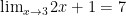
Figure 6 – As x approaches 3, 2x + 1 approaches 7.
From the table, we can clearly see that as the value of 
Mr. Jayson Dyer, author of The Number Warrior has another excellent explanation on the concept of limits in his blog Five intuitive approaches to teaching the infinitely small.
******
The area under the curve problem and the tangent problem are the ancient problems which gave birth to calculus. Calculus was independently invented by Gottfried Leibniz and Isaac Newton in the 17th century.