High School Algebra Archives - Page 2 of 31

Understanding Domain and Range Part 2

July 31, 2016 GB Calculus and Analysis, High School Algebra, High School Calculus, High School Mathematics

In the previous post, we have learned the graphical representation of domain and range. The domain of the function $f$ is the shadow or projection of the graph of $f$ to the x-axis (see the red segment in the figure below). The range of $f$ is the projection of the graph of $f$ to the y-axis (see the green segment in the figure below). In this post, we are going to learn how to analyze equations of functions and determine their domain and range without graphing.

domain and range

If a graph of a function is projected to the x-axis, the projection is the set of x-coordinates of the graph. A single point $(a,0)$ on the projection means a point on the graph exists. The existence of a point implies that $f(a)$ exists. This means that the function is defined at $x = a$ . In effect, the domain of a function is the set of x-coordinates that makes the function defined. In what follows, we learn some examples to illustrate this concept. » Read more

Leave a comment domain of a function examples, domain of a square root function, domain of functions, domain of rational function, getting the domain of a function, range of a function examples, range of functions

The Algebra and Geometry of Square Root

March 5, 2016 GB High School Algebra, High School Mathematics

If we have a square with a given area, then we can find the length of its side. For example, a square with area 4 square units has a side length of 2 units. In other words, in finding the side length of a square with area 4 square units,we are looking for a number that is equal to 4 when squared.The number that when squared is equal to 4 is called the square root of 4 and is written as $\sqrt{4}$ . From the discussion above, we now know that

$\sqrt{4} = 2$ .

It is easy to see that $\sqrt{1} = 1$ , since $1^2 = 1$ and $\sqrt{0} = 0$ since $0^2 = 0$ .

The square root of the two numbers above are integers, but this is not always the case. For instance, $\sqrt{2}$ is clearly not an integer since $1^2 = 1$ and $2^2 = 4$ . This means that $\sqrt{2}$ is somewhere between 1 and 4. What about $\sqrt{5}$ ? » Read more

Leave a comment area of a square, side length of a square, square of a number, square root of a number

The effect of adding b to the linear function y = ax + b

November 30, 2015 GB High School Algebra, High School Mathematics

In the previous post, we have learned about the effects of a in the linear function with equation y = ax. In this post, we learn about the effects of adding b to that equation. That is, we want to learn the effects of b in the linear function with equation y = ax + b.

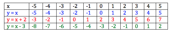
Consider the graph of the functions y = x, y = x + 2 and y = x – 3. The table of values (click figure to enlarge) below shows the corresponding y values of the three linear functions. The effect of adding 2 to the function y = x adds 2 to all the y values of y = x. This implies that in the graph, all the points with corresponding x values are moved 2 units above the graph of y = x. In addition, in the graph of y = x – 3, the -3 subtracts 3 from all the y values of y = x. In effect, all the points with corresponding x values are moved 3 units below the graph of y = x.

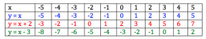
In addition, for y = x, if x = 0, y = 0. That means that the graph passes through the origin. On the other hand, for y = x + 2, when x = 0, then y = 0 + 2 = 2. This means that the graph passes through y = 2. Further, for y = 0 – 3 = -3. This means that the graph passes through y = -3. These are shown both in the table above and in the graph below. » Read more

Leave a comment linear function, y intercept, y intercept of a linear function

« 1 2 3 4 … 31 »