Note: This is the third part of the Derivative Concept Series. The first part is The Algebraic and Geometric Meaning of Derivative and the second part is Derivative in Real Life Context.
Introduction
The computation of derivative is often seen in maximum and minimum problems. In this article, we will discuss why do we get the derivative of a function and equate it to 0 when we want to get its maximum or minimum. To give you a concrete example, let us consider the problem below.
Find the maximum area a rectangle with perimeter 10 units.
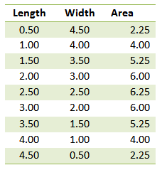
Without using calculus, we can substitute values for the rectangle’s length, compute for its width and its corresponding area. If we set the interval to 0.5, then we can come up with the table shown in Figure 1.

Figure 1 - Table showing the length, width, and area of a rectangle with perimeter 10.
Looking at the table above, we can observe that a rectangle of length of 2.5, a square, has the maximum area. If we have prior calculus knowledge, however, we know that whatever the value of our perimeter, a square having the given perimeter will always have the maximum area.
Using elementary algebra, if we let  be the width of our rectangle, it follows that the length is
  . Let
. Let  be the area of the rectangle. In effect, the area of the rectangle is described by the equation
  . We want to maximize the area, which implies that we want to find the maximum value of
  .
.

Figure 2 – A rectangle with Perimeter 10 and width x units.
In elementary calculus, to compute for the maximum value of  , we get its derivative, which is equal to
  , which we will denote
  . We then equate the
  to
to  resulting to the equation
  which is exactly the maximum value in the table above.
Derivative and Equation to 0
In the article the Algebraic and Geometric Meaning of Derivative, we have learned that the derivative of a function is the slope of the line tangent to that function at a particular point. From elementary algebra, we also have learned the properties of slopes. If a line is rising to the right, the slope is greater than 0; if the line is rising to the to the left, then the slope is less than 0. We have also learned that a horizontal line has slope 0 and the vertical line has an undefined slope.

Figure 3 – Properties of slope of a straight line.
In the problem above, we calculated by getting the derivative (the slope of the line tangent to a function at a particular point) and equate it to  . But a line with slope
  is a horizontal line. In effect, we are looking for a horizontal tangent of
  . To give a clearer picture let us look at the graph of
  .
.

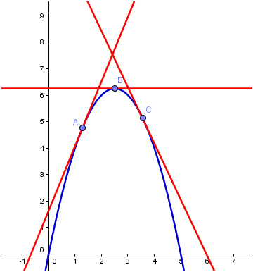
Figure 4 – Tangent lines of 5x – x2.
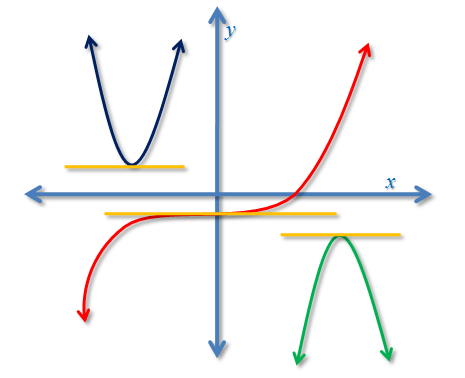
From the graph it is clear that the maximum point of the function is where the tangent line (red line) horizontal. In fact, there are only three possible cases that tangent line could be horizontal as shown in Figure 5: first, the minimum of a function (blue graph); second, the inflection point (red graph); and the third is the maximum of the function (green graph).
It should also be noteworthy to say that all the ordered pairs (length, area) or(width, area) in Figure 1 will be on the blue curve in Figure 4.

Figure 5 – Cases of a graph where the tangent is horizontal.
The derivative has many applications and it is seen in many topics in calculus. In the next Derivative Tutorial, we are going to discuss how the derivative is used in other context.
Summary
- The derivative of a function is the slope of the line tangent to a function at a particular point.
- The horizontal line has slope zero.
- In solving maxima and minima problems, we get the derivative of a function and equate to zero to get the minimum or maximum. We do this because geometrically, we want to get the line tangent to a function at a particular point that is horizontal.
is the derivative of
with respect to
and
is the second derivative of y with respect to x or in simpler terms, it is the derivative of
. » Read more

