GeoGebra Tutorial 19 – Basic Spreadsheet Recording

This is the 19th tutorial of the GeoGebra Intermediate Tutorial Series. If this is your first time to use GeoGebra, you might want to read first the GeoGebra Essentials Series.

A spreadsheet is a program that can be used to organize data in tables and  perform mathematical computations. Recently, GeoGebra integrated spreadsheet in its graphical user interface. In this tutorial, we learn how to use the GeoGebra spreadsheet.

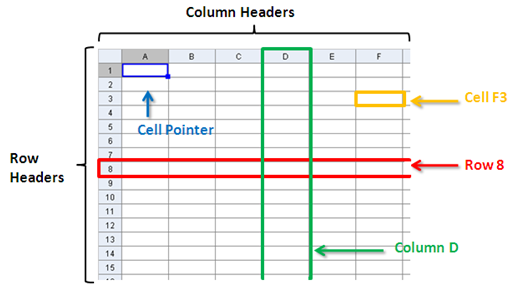
Figure 1

The figure above shows the different parts of a spreadsheet.  The following are the descriptions. You should familiarize yourself with these terms because we are going to use them in this tutorial and the two more tutorials to come. » Read more

GeoGebra Tutorial 18 – Area Under a Curve and Riemann Sums

This is the 18th tutorial of the GeoGebra Intermediate Tutorial Series. If this is your first time to use GeoGebra, I strongly suggest that you read the GeoGebra Essentials Series.

In this tutorial, we compare the area of a plane under a curve f(x) = x2 bounded by the x-axis, the y-axis, and the line x = 1 with the sum of the areas of rectangular partitions under the same boundaries.  We use the Slider tool to increase the number of rectangles and observe how they relate to the actual area.

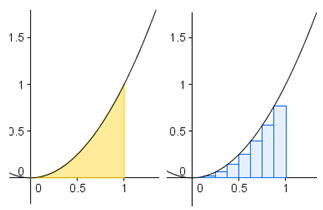
Figure 1 – Actual and approximate area bounded by the curve, the x-axis and x=1

If you want to follow this tutorial step-by-step, you can open the GeoGebra window in your browser by clicking here.  You can view the output of this tutorial here.

1. Open GeoGebra and select Algebra and Graphics from the Perspectives menu.
2.  Graph f(x) = x2 by typing f(x) = x^2 in the Input bar and press the ENTER key on your keyboard.
3. We now create a slider for the number of rectangles. Select the Slider tool and click on the Graphics view.

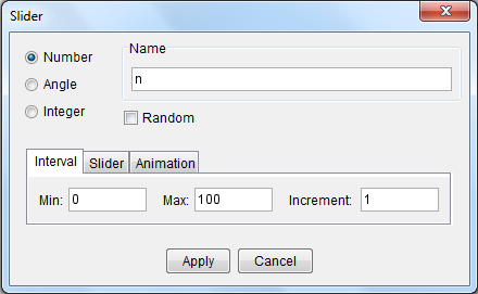
In the Slider dialog box, change the name to n, set the minimum to 0, maximum to 100, and increment of 1, then click the Apply button.

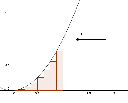
6. To construct the lower sum (rectangles whose upper left corners are on the curve), type lowersum[f,0,1,n] and then press the ENTER key on your keyboard.  That is, the lowersum (sum of the areas of rectangles) under the function f from 0 to 1 with number of rectangles.

Figure 3 – Approximate area with n = 8.

7. Move Slider n. What do you observe? Move n to the extreme right. What is the value of the lower sum or the total are of the rectangles under the curve?
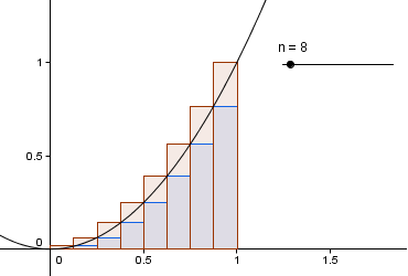
8. To construct the upper sum, type uppersum[f,0,1,n] in the drawing pad, and press the ENTER key.
9. Right click a (the value of the lowersum) in the Algebra window, and click Object Properties to show the Preferences window.
10. In the Preferences window, select the Color tab, choose a different color, then click the Apply button. This will make it easier to distinguish the two sums.

Figure 4 – Approximate area of the lower sum and the upper sum.

11. Move the slider to 100. What do you observe about the values of the the upper sum and the lower sum. Explain why your observation is such.
12. To get the actual area under the curve, we need the integral of the function f from 0 to 1. To do this, type integral integral[f, 0, 1] in the Input bar, and press the ENTER key.
13. Next, we construct a check box that will show/hide the three objects. To do this, select the Check box tool and click anywhere on the Graphics view.
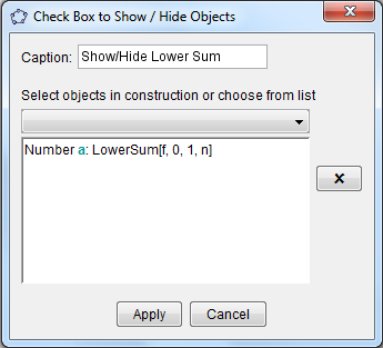
14. In the Caption text box, type Show/Hide Lower Sum, select Number a: Lower Sum[f,0,1,n] in the Select objects… box, and then click the Apply button.


15. Using steps 13-14 to create two more Show/Hide Check boxes for the Upper Sum and the actual area (integral of f from 0 to 1).
16. How are the lower sum, upper sum and area under the curve related?
17. How are the upper sum and lower sum related to the number of rectangles?

GeoGebra Tutorial 17 – Functions, Tangent Lines and Derivatives

This is the 17th tutorial of the GeoGebra Intermediate Tutorial Series. If this is your first time to use GeoGebra, I strongly suggest that you read the GeoGebra Essentials Series.    In this tutorial, we are going to use slider control a, b, c, d and e and graph the function f(x) = ax4 + bx3 + cx2 + dx + e.

Figure 1

We then  construct a line tangent to the function and passing through  point A and trace the graph of the point whose x-coordinate is the x-coordinate of A, and whose y-coordinate as the  slope of the tangent line. We compute for the derivative of f(x), and see if  there is a relationship between the trace and the derivative. If you want to follow the this tutorial step by step, you can open the GeoGebra window. Before following the tutorial, you may want to see the final output.

1. Open GeoGebra. We will need the Algebra view and the Axes so be sure that they are displayed. If not, use the View menu from the menu bar to show them.
2. To label points only, click the Options menu, click Labeling, and then click New Points Only.
3. To create slider a, type a = 1 in the input box and press the ENTER key. Right click the equation a = 1 in the algebra window (leftmost window pane) and click Show object from the context menu. Slider a should appear on your drawing pad.
4. Using step 3, create 4 more sliders namely b, c, d and e.
5. To graph the function f(x) = ax4 + bx3 + cx2 + dx + e, type f(x) = a*x^4 + b*x^3 + c*x^2 + d*x + e in the input box, then press the ENTER key.
6. Move the sliders and observe what happens.
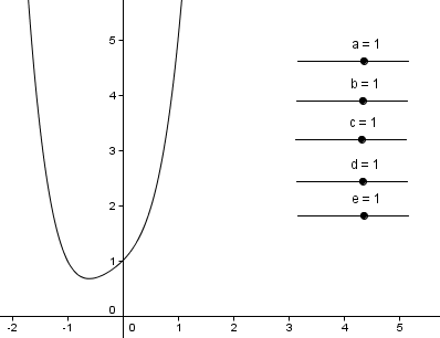
Figure 2

7. To construct point A on function f, select the New Point tool and click graph of the function.
8. To construct a line tangent to f and passing through A, select the Tangents tool, click point A and click the graph of f. A tangent line should appear passing through point A.
9. Move point A on the function, and move the sliders. What do you observe?
10. To get the slope of the tangent line, select the Slope tool and then click the tangent line. This will produce m (see Algebra window). Given similar values of the numerical coefficients and the right place for point A, your graph should look like Figure 3.

Figure 3

11. We now create point D, which will trace the ordered pair (x(A),m) where m is the slope of the tangent line. Note that x(A) means the x-coordinate of A and m was automatically assigned by GeoGebra to the value of the slope.  To create the point type D = (x(A), m).
12. We now change the color of point D. To do this, right click point D, and click Object Properties from the context menu. In the dialog box, select the Color tab and select a color you want from the color palette. Next, select the Basic tab, be sure to check the Show trace check box, then click the Close button.

Figure 3

13. Move point A along the function. What do you observe about the traces of point D?
14. To graph the derivative of f(x), type f’(x) = derivative[f], then press the ENTER key. What do you observe about the derivative of the function f?
15. Right click the derivative function and click Properties. In the dialog box, go to the Color tab and select the color you want, preferably the same color as point D. Drag point A. After this step, your drawing should look like the one shown in Figure 1.
16. What can you say about the relationship of the derivative and the path traced by point D and the derivative function?
17. How can you relate the tangent function, its slope, the derivative function and the line traced by point D?
18. Based on the activity above, how will you describe the derivative of a function at a particular point and derivative in general?
1 34 35 36 37 38 44