Rational and Irrational Numbers
The need of men to perform certain mathematical operations led to the birth of different types of numbers. People in the ancient times used only counting numbers to keep track of the number of their belongings such as animals. The concept of trade led to the invention of 0 and negative numbers. The need to divide led to the invention of rational numbers.
In this article, we are going to take a look at the characteristics of rational and irrational numbers.
Rational numbers are numbers of the form a/b where a, b are integers, and b not equal to zero. Rational numbers are called rational not because they are reasonable, but because they are a ratio of two integers. It is worthy to note the conditions in the definition. That is because not all fractions are rational numbers. For example, 
Geometric Interpretation of Rational and Irrational Numbers
In ancient times the Greeks, particularly the Pythagoreans, believed that all quantities are rational; that is, all quantities can be expressed as a ratio of two integers. Geometrically, this can be interpreted as follows. Given any two lengths, a unit length can be found that can measure the two lengths exactly without gaps or overlaps. In the example in Figure 1, we have two segments a and b, and we found a unit length that would fit exactly a whole number of times in both segments. The ratio of a:b is 7:6, or we can express it in a fraction that a is 7/6th of b.

Figure 1 – The division of segments a and b into unit lengths.
This belief, as most of us now know, was proven to be false. The Pythagoreans later discovered that given a square with length 1 unit, no unit length, however short, can be found to measure both the side of the square and its diagonal like what we have done above. They have concluded that the length of the diagonal cannot be expressed as the ratio of two integers and hence not rational. Today, numbers that are not rational are called irrational numbers. Hence, we define irrational numbers as numbers that cannot be expressed as a ratio of two integers.

Figure 2 – The square with length 1 unit has irrational diagonal.
Using the Pythagorean Theorem, we now know that the length of the diagonal of a square with side length 1 unit is equal to 
The collection of all rational and irrational numbers is called real numbers. Geometrically, real numbers are represented by the real line as shown in Figure 3.

Figure 3 – The real number line.
Each real number can be represented by a point on the real number line and every point on the number line has a corresponding real number.
Another Representation of Rational and Irrational Numbers
Aside from fractions, we can also represent rational numbers with decimals. For example, 1/5 = 0.2 and 1/3 = 0.333…. Observe that 0.2 has a finite number of decimals while 0.333… has infinite. Irrational numbers can also be represented using decimals. They are the types of decimals that do not end and do not repeat.
Several irrational numbers are very popular, and we had been using them from elementary school to college. The irrational numbers 


Figure 4 – The structure of the real number system.
From our discussion above, we can see that real numbers are divided into two main subsets – rational and irrational numbers.


 definition of limits. The definition says that the
  if and only if, for all
  , there exists a
  such that if
  , then
 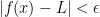 . In this article, we are going to discuss what this definition means. Readers of this article must have knowledge about elementary calculus and the
  . We have learned from elementary calculus that
  . Aside from algebraic computation, this is evident from the color-coded graph and the table shown in Figure 1. The yellow arrows in the graph and the values in the yellow cells in the table indicate that as the value of
  approaches
  from the left of the x-axis, the value of
  approaches
  from below of the y-axis. On the other hand, the red arrows in the graph and the values in the red cells in the table indicate that as the value of
 (with
(with  nines) to get an
  (
( nines).
 with (
 nines. This can be repeated for every chosen distance.
 ) from
  ) from
  and
and  , then
  and
and  .
. then the interval of our
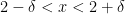
  . The definition of limit says that given a distance
  , we can find a distance
  and
and  . We do not know the value of
 . Subtracting
 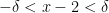 . If you recall the definition of absolute value, this is precisely the same as
  . The comparison among the notations is in Table 1.
 , then
  , then
 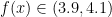 .
. .
. , then
  .
. . Our next task is to find the
  (any distance from x to the left and right of
  .
. and
and  be the fixed value that
  if and only if, for any
  (any small distance from to the left and to the right of a) such that if
  then,
then,  . And that is precisely, the definition of limits that we have stated in the first paragraph of this article.
 . In addition, the phrase “we can find” is also the same as “there exists” and is denoted by the symbol
  . So, rephrasing the definition above, we have
  , such that if
  , such that
  . The symbol
  stands for if and only if and the symbol
  is similiar to if-then. If
  and
and  are statements, the statement
  is the same as the statement of the form “If
  (any small distance above and below 4),
  such that if
  then,
then,  . This implies that
 which implies that
  . Simplifying, we have
  . This means that our
  and
and  to be sure that our
 . This means that our interval is
  . Now
. Now  . Thus,
  which implies that
  . Solving, we have
  . This means that our
  and
and  to be sure that our
  and
and  . There are only two examples above, but the definition tells us that we can choose any
  . Solving, we have
  . From the condition above,
  .
. and we are sure that if
  and
and  to be sure that our