distance formula Archives - Math and Multimedia

Math and Multimedia Carnival Criteria for Selection of Articles

July 21, 2010 GB Blog Carnival, High School Mathematics

The Mathematics and Multimedia Blog Carnival is now accepting articles for the next issue. Although any math article might be accepted, below are the Revised Criteria for Blog Carnival Selection. This will be characteristics of the articles that will be prioritized. Articles with no links are done, but not yet posted.

1. Connection between and among different mathematical concepts

2. Connections between math and real life; use of real-life contexts to explain mathematical concepts

3. Clear and intuitive explanation of topics not discussed intextbooks, hard to understand, or difficult to teach

4. Proofs of mathematical theorems in which the difficulty of the explanation is accessible to high school students

5. Intuitive explanation of higher math topics, in which the difficulty is accessible to high school students

6. Software introduction, review or tutorials

7. Integration of technology (Web 2.0, Teaching 2.0, Classroom 2.0), in teaching mathematics

Using Google Sketchup in Teaching Mathematics
Use of Google Docs in Teaching Mathematics.

Mathematics and Multimedia Blog Carnival is still in its infancy, so please help spread the word about it. I would appreciate if bloggers who has benefitted from Mathematics and Multimedia, especially those whose article was accepted in the previous carnival, would announce it in their blogs.

To submit article the Math and Multimedia Blog Carnival, click here.

The Math Teachers at Play Carnival and Carnival of Mathematics are also accepting math articles for their carnivals. Please do not duplicate submissions.

Erlina Ronda of Keeping Mathematics Simple will host the Mathematics and Multimedia blog carnival special edition on December 2010. Her topic will be on Teaching Algebra Concepts. You can email her to submit in advance.

—

Photos: Wikipedia Concept Map by juhansonin, Mandelbrot Julia Section by Arenamontanus

12 comments blog carnival, counting the real numbers, definition of undefined, distance formula, division by 0, GeoGebra Tutorial Series, google sketchup, incommensurables and irrational numbers, infinitude of primes, introduction to limits, investigating polyhedrons, is 0.999… = 1, lore of large numbers, mathematics and multimedia, pythagorean theorem, rational and irrational numbers, tessellation

Pythagorean Theorem, Distance Formula, and Equation of a Circle

July 19, 2010 GB High School Geometry, High School Mathematics

In my Algebraic and Geometric Proof of the Pythagorean Theorem post, we have learned that a right triangle with side lengths $a$ and $b$ and hypotenuse length $c$ , the sum of the squares of $a$ and $b$ is equal to the square of $c$ . Placing it in equation form we have $c^2 = a^2 + b^2$ .

If we place the triangle in the coordinate plane, having $A$ and $B$ coordinates of $(x_1,y_1)$ and $(x_2,y_2)$ respectively, it is clear that the length of $AC$ is $|x_2 - x_1|$ and the length of $BC$ is $|x_2 - x_1|$ . We are finding the length, which means that we want a positive value; the absolute value signs guarantee that the result of the operation is always positive. But in the final equation, $c^2 = |x_2 - x_1|^2 + |y_2-y_1|^2$ , the absolute value sign is not needed since we squared all the terms, and squared numbers are always positive. Getting the square root of both sides we have,

$c = \sqrt{|x_2 - x_1|^2 + |y_2-y_1|^2}$

We say that $c$ is the distance between $A$ and $B$ , and we call the formula above, the distance formula. » Read more

11 comments conic sections equation of a circle, derive equation of a circle, distance formula, equation of a circle, equation of a parabola, find equation of a circle, hypotenuse of a right triangle, pythagorean theorem, pythagorean theorem example, pythagorean theorem formula, pythagorean theorem proof, right triangles

A Closer Look at the Midpoint Formula

January 20, 2010 GB High School Algebra, High School Geometry, High School Mathematics

Introduction

If we want to find the midpoint of segment CD in Figure 1, where the coordinates of points C and D are $(-2,5)$ and $(-2,1)$ , it is clear that the length of CD is $5 - 1 = 4$ units. To determine the midpoint of CD, we want to get the coordinates of the point which is $2$ units away from both points C and D. Hence, we have to divide $5 - 1 = 4$ by $2$ , and add the result to $1$ or subtract the result from $5$ . Summarizing, the expression that would describe the value of the y-coordinate of the midpoint would be $\displaystyle\frac{(5 - 1)}{2} + 1$ or $5 - \displaystyle\frac{(5 - 1)}{2}$ . This means that the midpoint of CD is $(0,2)$ .

If we want to get the midpoint of AB, using the same reasoning above, the expression that would describe the x-coordinate of the midpoint would be $\displaystyle\frac{(6 - 3)}{2} + 3$ or $6 - \displaystyle\frac{(6 - 3)}{2}$ . This means that the midpoint of AB is $(1.5,0)$ .

Figure 1 – Horizontal line AB and vertical line CD in the coordinate plane.

Generalizing our observation above, if we have a vertical segment with their endpoints having coordinates $(a, y_1)$ and $(a,y_2)$ (see Figure 2), we can get its midpoint using the following formula $\displaystyle\frac{y_2 - y_1}{2} + y_1$ or $y_2 - \displaystyle\frac{y_2 - y_1}{2} + y_1$

Figure 2 – Generalized coordinates of a vertical and a horizontal line.

Simplifying, both the expressions above result to $\displaystyle\frac{y_2 + y_1}{2}$ . Similarly, for a horizontal segment with endpoints having coordinates $(x_1, b)$ and $(x_2, b)$ can be computed by the expression $\displaystyle\frac{x_1 + x_2}{2}$ .

Midpoint of a Slanting Segment

The preceding derivations are only valid for vertical and horizontal segments. In Figure 3, segment AB is neither horizontal nor vertical. To investigate the midpoint of AB, we draw vertical segment PQ coinciding with the y-axis with endpoints having y-coordinates the same as those of the y-coordinates of segment AB (see Figure 3). We also draw a horizontal line RS coinciding the x-axis with endpoints having x-coordinates the same as those of the x-coordinates of segment AB. Looking at Figure 3, it is clear that the coordinates of the midpoint of the PQ is $(0,3)$ .

If we draw a horizontal line from $(0,3)$ towards segment AB (see yellow dashed segment), and draw a vertical line from the intersection M to segment RS, it seems that the intersection of the yellow dashed line and segment RS is $(3.5,0)$ which is the midpoint of RS. From here, it is tempting to ask the following question:

“If the midpoint of PQ is $(0,3)$ and the midpoint of RS is $(3.5,0)$ , is the midpoint of AB, $(3.5,3)$ ?

Figure 3 – A non-horizontal segment AB with midpoint M.

Generalizing the questions above, we might want to ask “If the midpoint the point with coordinates A $(x_1,y_1)$ and B $(x_2, y_2)$ equal to $(\displaystyle\frac {x_1 + x_2}{2}, \displaystyle\frac{y_1 + y_2}{2})$ ?”

If we extend the QA and the horizontal yellow dashed line to the right, we can from two right triangles as shown in Figure 4. From the statements above, we want to show that point M is the midpoint of AB.

To show that M is the midpoint of AB, it is sufficient to show that AM is congruent to MB. This leads us to Figure 5, where we label the right angles of the two triangles T and U. We will now show that triangle AUM is congruent to triangle MTB. If so, then we can show that AM is congruent to MB since they are the corresponding sides of the given triangles.

Proof that AUM is congruent to MTB

Since PB and MT are horizontal segments, we can consider AB as a transversal of parallel segments PB and the segment containing MT. It follows that angle TBM and angle UMA are congruent because they are corresponding angles. It is also clear that BT is congruent to MU, and angle T is congruent to angle U since they are both right angles. Therefore, by the ASA congruence theorem, AUM is congruent to MTB. (For an explanation of parallel lines and transversals, click here).

Since corresponding parts of congruent triangles are congruent, AM is congruent to MB. Hence, M is the midpoint of AB.

Figure 5 – The triangle produced by extending the horizontal lines passing through the three points.

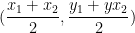Note that our proof did not talk about coordinates, but the general case. That is, if the coordinates of A are $( x_1, x_2)$ and the coordinates of B are $(y_1, y_2)$ , the coordinates of M is equal to $(\displaystyle\frac{x_1 + x_2}{2},\displaystyle\frac{y_1 +yx_2}{2} )$ .

Delving Deeper

There are also other ways to show that the midpoint of AB is M. $( x_1,y_1)$ and $( x_2,y_2)$ lies on the midpoint formula. The details of the solutions are left to the reader as an exercise.

From Figure 3, draw two right triangles with hypotenuse AM and hypotenuse AB and show that AM is half of AB.
Using the distance formula, show that the distance between point A and point M is the same as the distance between point M and point B.
Show that AM and MB has the same slope.
Get the equation of the line containing AB, and substitute the coordinates of M to the equation of line AB.

3 comments ASA congruence theorem, congruent angles, congruent triangles, congruent triangles geometry, congruent triangles math, coordinate geometry, coordinate geometry midpoint formula, derivation of the midpoint formula, distance formula, geometry parallel lines and transversals, linear measure midpoint formula, midpoint formula, midpoint formula geometry, midpoint line segment formula, side angle side